Lab Four: GPS and GIS - Using Control Points Collected in the Field to Georeference a .jpg of the UCCS Campus
Lab Four Goals (READ CAREFULLY)
- to extend GPS into GIS
- to recognizie the value of primary data
- to gain experience georeferencing in a GIS (in our case, aligning a non-georeferenced plan-view photo using GPS lat./long. pairs)
- to learn how to prepare a spatial database (with attributes) for import into GIS software
- to learn how to import x, y data from Excel into ArcMap
- to understand the concept of ground control points, such as sidewalk intersections and parking lot corners
- to learn how to 'rubber sheet' an image using control points
Background (READ CAREFULLY)
Downloadable raster images, such as the ~55,000 US Geological Survey (USGS) DRGs, DEMs, DOQs, and GeoPDFs, contain imbedded georeferencing information. These georeferenced files, when opened in GIS software, are miraculously and mysteriously fixed to their appropriate geographic location on the Earth's surface. Images captured or 'snipped' from Google Earth, and primary image data, such as images you might collect using balloon or kite photography, contain no such spatially explicit data (e.g., they are not georeferenced) and are thus incapable of contributing to a GIS project in which other map layers are spatially stacked / aligned. However, following a few easy steps, any image with known ground control points (geospatially referenced ground markers) can be georeferenced in a GIS environment.
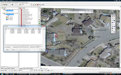
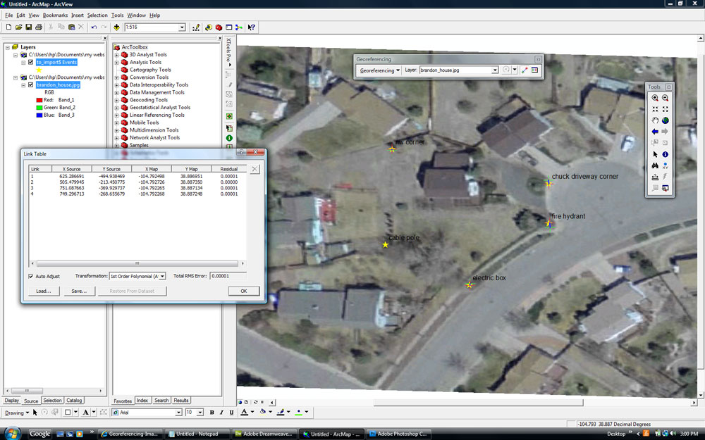
The homework assignment from a few weeks ago (we made this 'Lab Three') introduced you to the basics of ArcMap. Lab Four requires ArcMap's "Georeferencing tool" to georeference, or, to fit a map into a known coordinate system. With a few clicks of the mouse, the georeferencing tool guides the alignment of images to a known map coordinate system, which is defined by the map projection. Here is a screenshot from ArcGIS showing Brandon's house after georeferencing. The points are GPS locations that were 'rubber sheeted' or stretched into place on the map. How does this all happen? KEEP READING!
Overview (READ A COUPLE TIMES VERY CAREFULLY)
 Lab Four incorporates much of the content covered thus far in GES2050. Specifically, the lab brings together cartographic basics, raster and vector data models, file types, image editing, information presentation and delivery, and primary and secondary data. In Lab Four, these 'parts' coalesce as students work through a real-world problem that is easily addressed using GIS: georeferencing imagery. Students use GIS software to georeference a UCCS campus air photo according to student-collected GPS waypoints.
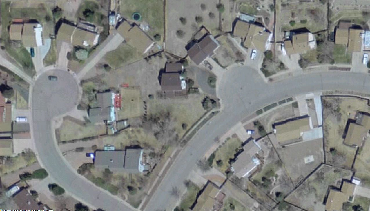
In Lab Four, students use Garmin ETREX global positioning system (GPS) receivers to collect and record ground control points (waypoints) at various locations across campus. In addition to collecting spatial data (GPS waypoints), students collect and record descriptive attribute information. The campus locations selected for control points (lat./long. coordinates) must be easily visible on the UCCS campus air photo exported from Google Earth or similar (here's an example of an image of Brandon's house that was exported from SkylineGlobe, a virtual globe that is similar in many ways to Google Earth). The control points collected should be located around the perimeter of the map, near the center of the map, as well as a couple randomly scattered throughout the mapping area.
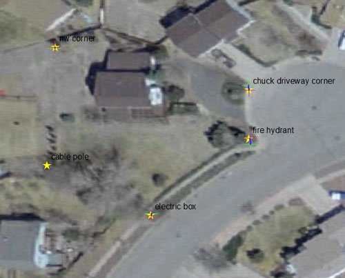
Control points provide a means to manually attach geospatially referenced data to the non-georeferenced UCCS campus air photo (here are the locations Brandon selected for his house. Oops! - he should have collected a couple points from the center of the property). Aligning an image (such as an image of the ground you might take from an airplane) to spatial data is achieved through a georeferencing process called 'rubber sheeting' in which a mouse is used to connect lat./long. points to the exact place on the image where the points were collected in the field. The spatial lat./long. point data and the non-spatial attribute information describing the location of the points will be imported into ArcMap via a MS Excel worksheet table. After georeferencing the campus map, the map layer becomes a useable layer for a GIS project. For example, with a 'snipped' overhead view Google Earth campus photo, it becomes possible to overlay existing map layers (secondary data), such as USGS DRGs, DEMs, and DOQs, and to digitize/create new Shapefile features (points, lines, polygons) from the map. Pretty cool, eh? This is a common task performed in GIS software.
Due Sunday, Mar. 24, 5:00 pm
Tools
- Garmin ETREX GPS receiver
- Garmin BaseCamp
- MS Excel worksheet
- ESRI ArcMap GIS Software 10.6
- MS Expression Web 4
- Filezilla
- File compression (built in to Windows 10)
- A web browser
STEPS TO COMPLETE LAB FOUR
READ THE "WHAT I GRADE" SECTION BELOW RIGHT NOW - YOU WILL NEED TO SAVE FOUR SCREEN SHOTS FROM THE STEPS BELOW
1) Geospatial database preparation
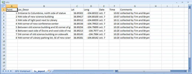
- VERIFY that your spatial (lat./long.) and non-spatial (attribute) data, which are stored in your group's Excel file, are indeed ready for import into GIS software. This is a critical step in the process! Remember: Garbage in, garbage out (GIGO). To check, open up the Excel file that contains your waypoints and attribute information with no formatting (no formulas, no cell outlines, no bold text, etc.). When the data on your worksheet look something like this, close Excel.
2) Into ArcMap, import Excel database and .jpg campus map
- Open ArcMap. When the little window pops up asking what you want to open, select "Blank Map" and click 'ok'.
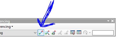
- In ArcMap, turn on (check) the "Georeferencing toolbar" (Customize > Toolbars > Georeferencing). This tool will allow you to georeference your campus map.
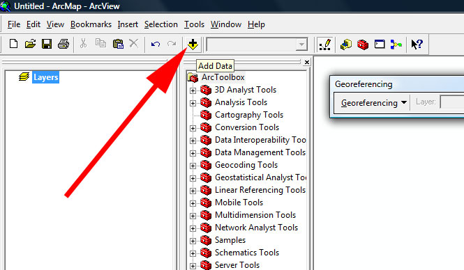
- In ArcMap, open up the Arc Toolbox window (click the little icon with the red toolbox to do this). ArcToolbox is your friend - as you already know, it is the way to access most tools that ArcMap provides.
- Next, in ArcMap, add to your project the campus map (the digital form of the hard-copy you carried around campus as you collected waypoints). This image can be found in Canvas (modules > Digital Image of Campus (for Lab Four) > uccs_ge.jpg). First, save the image to your lab four directory. To add the image to ArcMap project, click the little 'Add data' icon and navigate to the campus .jpg map. NOTE: As was demonstrated in class a couple of weeks ago, you will first need to use the "Connect to Folder" icon to connect to your ges2050 directory (the 'Connect to Folder' icon is in the 'Add data' box - it's the little folder with the black '+' sign on it)
- After adding the .jpg, you might be asked if you want to "Create pyramids for...?," say yes -- and leave all of the defaults.
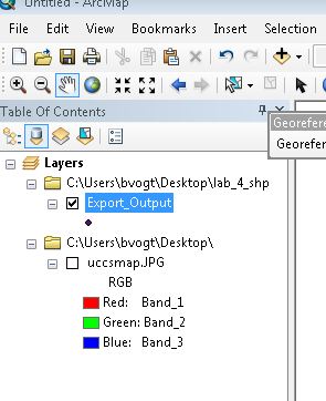
- Also, you will receive an "Unknown Spatial Reference" error, click okay - we know this - this is what we are trying to fix! Your view should now look something like this.
- Next, let's import your GPS data (from the Excel file).
- In ArcMap, click the 'Add data' icon again (like you did to add your campus map) and navigate your group's Excel file
- Double-click on the .xlsx file. If you get a 'Connect' error that says 'Failed to connect to database,' you will need to save your Excel file as an .xls (from a .xlsx) and then repeat this step (this is one of those quirks in ArcMap - it sometimes likes 'older' versions of other softwares, including Excel).
- Within the Excel file, add (double-click on) the worksheet you named 'to_import'
- You should now see the worksheet's name (to_import) in the Table of Contents in ArcMap. In the Table of Contents, RIGHT click on the new map layer and select 'Display XY Data'
- Because of the way Garmin's BaseCamp named the fields (columns are called 'fields' in ArcMap) in your Excel worksheet, ArcMap knows to assign 'x' to lon and 'y' to lat (we'll ignore the 'ele' - leave 'ele' as <None>). DO NOT CLICK 'OK' YET!
- Next, in the 'Display XY Data' window, you must assign the GPS coordinates a coordinate system: Click the little "edit" button in the "Display X,Y Data" window and navigate as such:
- Select > Geographic Coordinate System > North America > USA and territories > NAD 1983. Click Add and then click OK, OK.
- You'll see a warning that says: 'Table Does not Have Object-ID Field' (click OK - that's okay - we will address this soon)! You will probably NOT see any of the waypoints in your map view - don't worry.
- Notice that the process of adding NAD 1983 created a new map layer in the table of contents. This is VERY helpful because now we can view and edit attributes (attribute data, point size, point color, etc.). BUT we need an "Object ID" field, so we need to create a Shapefile from the map layer!
- Save your project as an 'Arc Map Document' (a .mxd file) somewhere to your Lab Four folder as "lab_4."
- To create a Shapefile, in the ArcGIS Table of Contents, right-click on the new map layer file. Go to >Data > Export Data.
- In the Export Data window, click on the yellow folder icon.
- Save as a Shapefile (.shp) -- Use the pulldown menu to change from 'File and Personal Geodatabase feature class' to 'Shapefile.' Use THE DEFAULTS but make sure the new 'Export_Output' Shapefile (ending in .shp) is saved to YOUR Z: DRIVE in your lab_4 folder! (you can leave the file naming alone; just use defaults).
- When asked if you want to add the exported data to the map, say yes.
- This is a good time to remove the map layers you no longer need: In the Table of Contents, right-click on map layers and select 'Remove.' Keep only the Shapefile and the campus image (map).
- Your image (.jpg campus map) and the GPS waypoints (Export_Output.shp) are now loaded in your GIS project. GREAT. But they are likely very far apart (spatially). Let's fix that.
- Turn off (uncheck) the campus map view (and leave the new GPS point Shapefile on and selected).
- Right-click on the Export_Output Shapefile and select 'Zoom to Layer' (you should see your points fill the display window; if not, zoom in on the set of points until they more/less fill the window. If needed, ask Brandon to help you delete bad waypoints (points that are far away from others in the group).
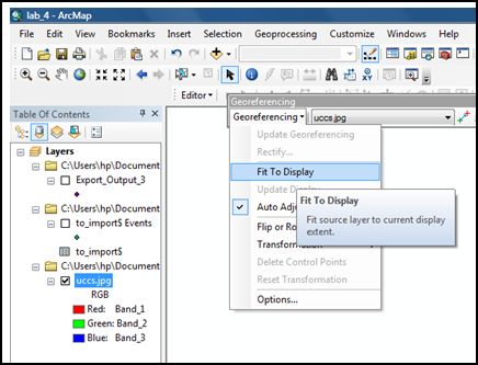
- Next, turn on (check the box) and select (so the campus map .jpg in the table of contents turns blue) the .jpg image and use the 'Georeferencing tool bar' tool called 'Fit to Display'. This should scale your GPS points and image very close to one another on your screen. If the alignment is poor, redo this step AFTER zooming in or out of your point shapefile so the points roughly fit the map window.
- Experiment with turning off and on the image and turning off and on the GPS points (the Shapefile you created). You may want to change the color of the GPS points to an ugly purple or yellow color and increase the size of the dot to something like 12 so you can see them on top of your campus image (double-click directly on the Shapefile's 'dot' icon in the table of contents to change symbol size, color, shape, etc).
- Add labels to your points: Right-click on the Shapefile and select 'Label Features'
- Turn on your Location Description (called something like 'cmt' or 'desc' in the attributes table) labels so you know which point will go where (right-click on the Shapefile and select 'Label features'). To change the 'label' field and its properties, double-click on the Shapefile from the Table of Contents (this opens the 'Layer properties' window) and adjust the settings as seen here. THIS IS ONE REASON WHY IT IS CRITICAL TO RECORD DESCRIPTIVE ATTRIBUTE LOCATION INFORMATION AT EACH OF YOUR WAYPOINT LOCATIONS
- NOW WE ARE READY TO ADD CONTROL POINTS (in other words, ATTACH YOUR GPS COORDINATES TO THE IMAGE)
3) The georeferencing process (please follow steps VERY carefully)
- From the 'Georeferencing tool', click the 'add control points' icon.
- Using your mouse, regular click (left click) on a known point on the campus image (the exact place you stood to collect a waypoint). This will place a cross mark on that location.
- Next, regular click (left) on the matching control point from the GPS point layer. This will actually move (stretch or rubber sheet) the image and better align the control points.
- Repeat the above
(image click, point click... image click, point click) for the remaining control points.
- Things might get crazy here: If you want to delete any of your links, open the 'View Link Table', select the bad link, and use the delete button on your keyboard to delete the link.
- Do you want to throw your computer out the window? Ask Brandon for help! If you have bad GPS data, this process will not work well or at all. If one of your waypoints is way off, your final map might end up looking like an M.C. Escher piece. Remember: GIGO (garbage in, garbage out). If you are totally stressed out because your image has become distorted beyond all recognition, feel free to use GPS waypoints (Excel file) from another group in class who did not have trouble georeferencing.
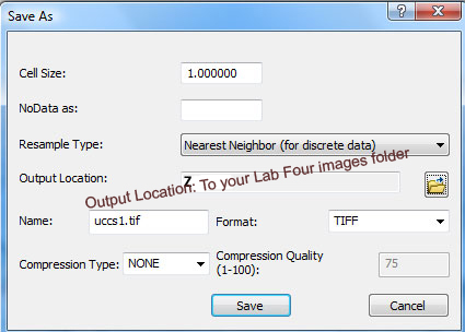
- When you are finished georeferencing your image to the waypoints, use the 'Rectify tool' (Georeferencing > rectify) to make your map permanently georeferenced (the 'Rectify tool' creates a 'world file' that contains georeferencing information).
- When using the rectify tool, FIRST CHANGE the Output Location (a folder) to your lab four DIRECTORY -- THEN you are able to change the format to 'TIFF'. Use all of the other defaults before you click 'Save'.
- Sing out loud 'GIS is SO MUCH FUN, SO MUCH FUN, SO MUCH FUN' (to the tune of the Mary had a Little Lamb)
4) Zip (compress) the .tif files into one file
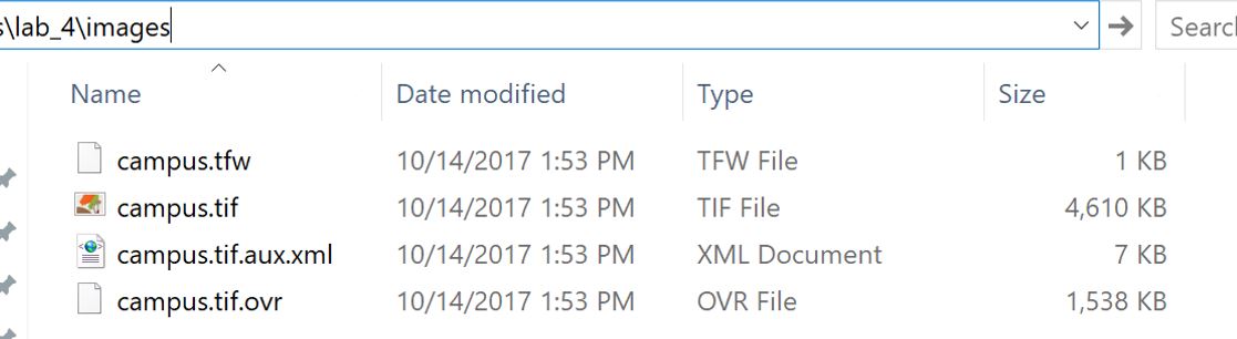
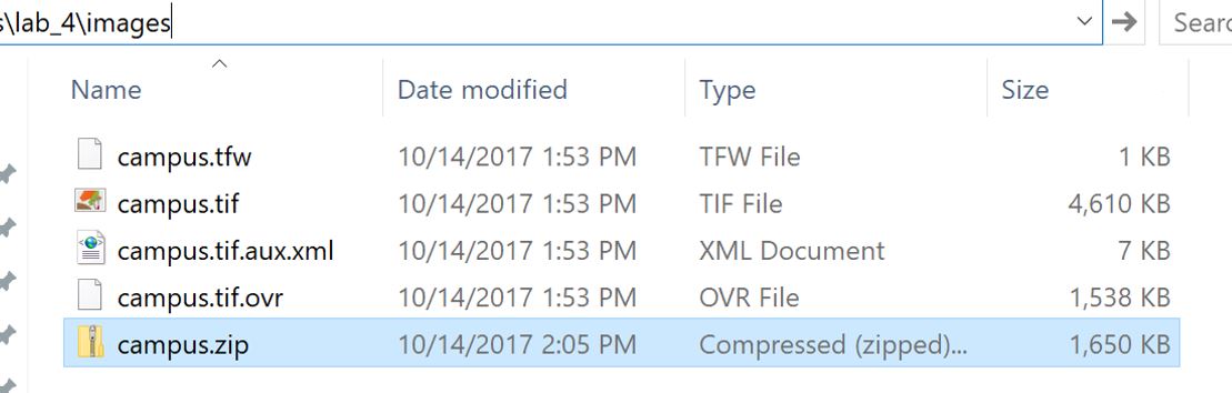
- When you rectified the image in the above step, a .tif (image file) was created. Along with the*.tif, a world file (we've talked about this a few times) was created (*.tfw), along with two other files, a *.tif.aux.xml and a*.tif.ovr.
- To grade your work, Brandon will need to open your georeferenced *.tif file map layer (which is actually four files) in ArcMap. Getting these files to Brandon is simplified if they are all compressed into one file. So we need to zip (or compress) these four files into one.
- Open the folder (that is stored on your z drive) containing the *.tif, *.tfw, *.tif.aux.xml, and *.tif.ovr.
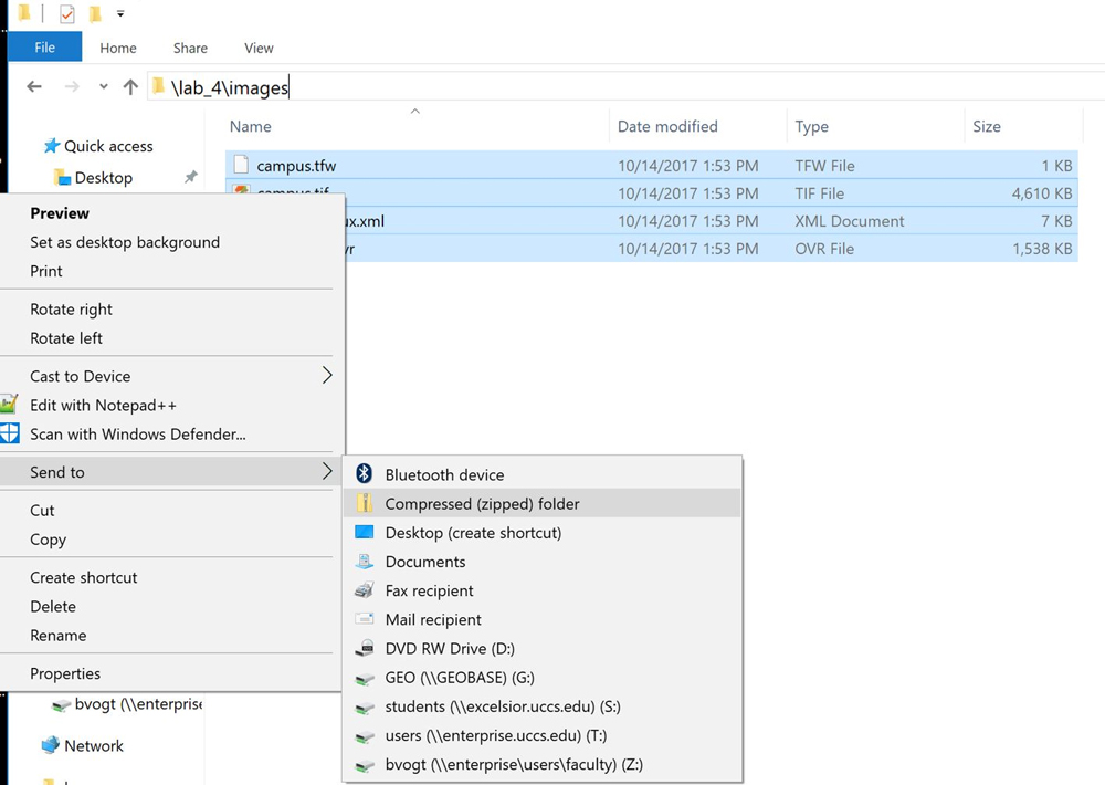
- Select all four of the files with your mouse.
- Right-click and select 'Send to > Compressed (zipped) folder'
- This process creates a zipped file (the icon looks like a folder - this one I named 'campus'). Note that the zipped folder is much smaller in terms of kb than the four uncompressed files that you zipped)! In this case, the zipped file is only 26% the size of the four unzipped files! Smaller is better when moving files around, storing them, and placing them on the internet. Another advantage is makingn ONE file from many!
- Now you have a zipped (compressed) folder on your z drive.
WHAT I GRADE:
-
Onto your Lab Four web page:
- Place any FOUR screen shots (snips) as .jpgs with captions from your ArcMap project that document any part of the georeferencing process.
- Place a link to the compressed (zipped) folder that contains the four files created when you rectified your map. NOTE: This is NOT a screen capture of the .tif; rather, it is a hotlink to the .tiff image, now stored in a zipped folder on your z drive AND on the 'coursework' web server. When I click on this link from your Lab Four web page, I will be able to view your rectified image in ArcMap. TEST THIS.
- ANSWER FOUR QUESTIONS (include the questions along with your answers):
- How are GPS and GIS related? Explain.
- What GIS-related problem(s) did you encounter in Lab Four?
- When georeferencing an image, why do you think it is important to collect detailed descriptive attribute information (non-spatial) along with the spatial information?
- Provide an example from your own interest area, or from another class you are taking / have taken, in which georeferencing an image could serve a useful purpose.