Section 3.1 Power Functions and Polynomial Functions
A square is cut out of cardboard, with each side having length $L$. If we wanted to write a function for the area of the square, with $L$ as the input and the area as output, you may recall that the area of a rectangle can be found by multiplying the length times the width. Since our shape is a square, the length & the width are the same, giving the formula:
$$A(L)=L\cdot L=L^2$$
Likewise, if we wanted a function for the volume of a cube with each side having some length $L$, you may recall volume of a rectangular box can be found by multiplying length by width by height, which are all equal for a cube, giving the formula:
$$V(L)=L\cdot L \cdot L=L^3$$
These two functions are examples of power functions, functions that are some power of the variable.
Power Function
A power function is a function that can be represented in the form
$$f(x)=x^p$$Where the base is a variable and the exponent, $p$, is a number.
Technically, the toolkit linear function $f(x) = x$ is a power function, since it can be written as $f(x) = x^1$. We’ll be studying some power functions with more interesting exponents in this chapter.
Toolkit Power Functions (Quadratic)
The toolkit power function with an exponent of 2 is
$$f(x)=x^2.$$
It is called the quadratic function.
This function is described by the following table and graph:
| $x $ | $ f(x)$ |
|---|---|
| $-2 $ | $ 4$ |
| $-1 $ | $ 1$ |
| $0 $ | $ 0$ |
| $1 $ | $ 1$ |
| $2 $ | $ 4$ |
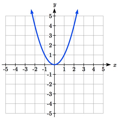
Features of the toolkit quadratic function
The quadratic function has the following features:
- Domain: $(-\infty,\infty)$
- Range: $[0, \infty)$
- Intercepts: $x$ and $y$ intercepts at (0,0).
- End behavior: As $x\to\infty, f(x)\to\infty$ and as $x\to-\infty, f(x)\to\infty$.
- Increasing on $(0, \infty)$
- Decreasing on $(-\infty, 0)$
- Concave up on $(-\infty, \infty)$
- Symmetric about the $y$-axis (even)
Toolkit Power Functions (Cubic)
The toolkit power function with an exponent of 3 is
$f(x)=x^3.$
It is called the cubic function.
This function is described by the following table and graph:
| $x $ | $ f(x)$ |
|---|---|
| $-2 $ | $ -8$ |
| $-1 $ | $ -1$ |
| $0 $ | $ 0$ |
| $1 $ | $ 1$ |
| $2 $ | $ 8$ |
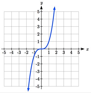
Features of the toolkit cubic function
- The cubic function has the following features:
- Domain: $(-\infty,\infty)$
- Range: $(-\infty,\infty)$
- Intercepts: $x$ and $y$ intercepts at (0,0).
- End behavior: As $x\to\infty, f(x)\to\infty$ and as $x\to-\infty, f(x)\to-\infty$.
- Increasing on $(-\infty, 0) \cup (0,\infty)$
- Symmetry: symmetric about the origin (odd)
Let’s spend a little time playing around with transformations of these functions.
Graph $g(x)=2(x-1)^2 + 4$ using transformation techniques. Then identify the domain, range, intercepts, end behavior, and intervals of increasing or decreasing. Finally, identify any symmetry present.
First, we look at the structure to determine our toolkit function. Here, we see that exponent of 2; that tells us we’re dealing with $f(x)=x^2$ as a parent. We want to identify $a, b, c$, and $d$ for $g(x)=af(bx+c) + d=a(bx+c)^2 + d$.
In this case, we have $a=2$, $c=- 1$, and $d=4$. We’ll use $c$ to shift the graph right 1, then use $a$ to vertically stretch by a factor of 2, and finally use $d$ to shift the graph up 4. In table form, that looks as follows.
| $X=x+1 $ | $ \leftarrow x $ | $ f(x)=x^2 \rightarrow $ | $y=2\cdot f(x) \rightarrow $ | $g(X)=y+4$ |
|---|---|---|---|---|
| $-1 $ | $ -2 $ | $ 4 $ | $ 8 $ | $ 12$ |
| $0 $ | $ -1 $ | $ 1 $ | $ 2 $ | $ 6$ |
| $1 $ | $ 0 $ | $ 0 $ | $ 0 $ | $ 4$ |
| $2 $ | $ 1 $ | $ 1 $ | $ 2 $ | $ 6$ |
| $3 $ | $ 2 $ | $ 4 $ | $ 8 $ | $ 12$ |
When we graph our transformed graph, we have this picture:

The function has the following features:
Domain: $(-\infty,\infty )$
Range: $[4, \infty)$
Intercepts: $y$ intercept at $(0,6)$. No $x$-intercepts.
End behavior: As $x\to\infty, f(x)\to\infty$ and as $x\to - \infty, f(x)\to\infty$.
Increasing on $(-\infty, 1) \cup (1,\infty)$
Symmetry: symmetric about the line $x=1$. Neither even nor odd.
In that example, we were using the graph of the function to identify our features. We could have used algebra to figure out things like the intercepts and whether the function was even or odd. Depending on what we want to do, sometimes graphing will be quicker, and sometimes algebra will be easier for determining these features!
Graph $$g(x)=\left( \frac{1}{2}x + 1 \right)^{3} - 1$$ using transformation techniques. Then identify the domain, range, intercepts, end behavior, and intervals of increasing or decreasing. Finally, identify any symmetry present.
This time we see that exponent of 3, which means we’re dealing with the toolkit function $f(x)=x^3$. We want to find $a, b, c$, and $d$ so that $g(x)=af(bx+c) + d=a(bx+c)^3 + d$.
We see $c=1$, so we start with a shift left 1. Then $b = \frac{1}{2}$, so there is a horizontal stretch by a factor of 2. Finally, $d=-1$, so the graph shifts down 1. We show this process in the following table and graph:
| $X\cdot \frac21 $ | $\leftarrow X=x-1 $ | $\leftarrow x $ | $ f(x)\rightarrow $ | $ y=f(x)-1$ |
|---|---|---|---|---|
| $-6 $ | $ -3 $ | $ -2 $ | $ -8 $ | $ -9$ |
| $-4 $ | $ -2 $ | $ -1 $ | $ -1 $ | $ -2$ |
| $-2 $ | $ -1 $ | $ 0 $ | $ 0 $ | $ -1$ |
| $0 $ | $ 0 $ | $ 1 $ | $ 1 $ | $ 0$ |
| $2 $ | $ 1 $ | $ 2 $ | $ 8 $ | $ 7$ |

The function has the following features:
Domain: $(-\infty,\infty )$
Range: $(-\infty,\infty )$
Intercepts: $x$ and $y$-intercept at $(0,0).$
End behavior: As $x\to\infty, f(x)\to\infty$ and as $x\to-\infty, f(x)\to-\infty$.
Increasing on $(-\infty, -2) \cup (-2,\infty)$
Symmetry: Neither even nor odd.
Graph $g(x)=-(x-2)^3-4$ using transformation techniques. Then identify the domain, range, intercepts, end behavior, and intervals of increasing or decreasing. Finally, identify any symmetry present.
Characteristics of Power Functions
Shown to the right are the graphs of $f(x)=x^2, f(x)=x^4$, and $f(x)=x^6$, all even whole number powers. Notice that all these graphs have a fairly similar shape, very similar to the quadratic toolkit, but as the power increases the graphs flatten somewhat near the origin, and become steeper away from the origin.
For all these even-powered power functions, we see the same end behavior: as $x\to\infty$, $f(x)\to\infty$ and as $x\to-\infty, f(x)\to\infty.$

Shown here are the graphs of $f(x)=x^3, f(x)=x^5$, and $f(x)=x^7$, all odd whole number powers. Notice all these graphs look similar to the cubic toolkit, but again as the power increases the graphs flatten near the origin and become steeper away from the origin.
For these odd power functions, as $x\to-\infty$, $f(x)\to-\infty$ and as $x\to\infty$, $f(x)\to\infty$.

Describe the long run behavior of the graph of $f(x)=x^8$.
Since $f(x)=x^8$ has a whole, even power, we would expect this function to behave somewhat like the quadratic function. As the input gets large positive or negative, we would expect the output to grow without bound in the positive direction. In symbolic form, as $x\to\pm\infty$, $f(x)\to\infty$.
Describe the long run behavior of the graph of $f(x)=-x^9$
Since this function has a whole odd power, we would expect it to behave somewhat like the cubic function. The negative in front of the $x^9$ will cause a vertical reflection, so as the inputs grow large positive, the outputs will grow large in the negative direction, and as the inputs grow large negative, the outputs will grow large in the positive direction. In symbolic form, for the long run behavior we would write: as $x\to\infty$, $f(x)\to-\infty$ and as $x\to-\infty$, $f(x)\to\infty$.
Describe in words and symbols the long run behavior of $f(x)=-x^4$
Polynomials
An oil pipeline bursts in the Gulf of Mexico, causing an oil slick in a roughly circular shape. The slick is currently 24 miles in radius, but that radius is increasing by 8 miles each week. If we wanted to write a formula for the area covered by the oil slick, we could do so by composing two functions together. The first is a formula for the radius, r, of the spill, which depends on the number of weeks, w, that have passed.
Hopefully you recognized that this relationship is linear:
$$r(w)=24+8w$$
We can combine this with the formula for the area, A, of a circle:
$$A(r)=\pi r^2$$
Composing these functions gives a formula for the area in terms of weeks:
$$A(w)=A(r(w))=A(24+8w)=\pi (24+8w)^2$$
Multiplying this out gives the formula
$$A(w)=576\pi +384\pi w+64\pi w^2$$
This formula is an example of a polynomial. A polynomial is simply the sum of terms each consisting of a vertically stretched or compressed power function with non-negative whole number power.
Terminology of Polynomial Functions
A polynomial is function that can be written as $f(x)=a_0+a_1x+a_2x^2+⋯+a_nx^n$
Each of the a_i constants are called coefficients and can be positive, negative, or zero, and be whole numbers, decimals, or fractions.
A term of the polynomial is any one piece of the sum, that is any $a_ix^i$. Each individual term is a transformed power function.
The degree of the polynomial is the highest power of the variable that occurs in the polynomial.
The leading term is the term containing the highest power of the variable: the term with the highest degree.
The leading coefficient is the coefficient of the leading term.
Because of the definition of the “leading” term we often rearrange polynomials so that the powers are descending.
$$f(x)=a_nx^n+.....+a_2x^2+a_1x+a_0$$
End Behavior of Polynomials
For any polynomial, the end behavior of the polynomial will match the end behavior of the leading term.
Identify the degree, leading term, and leading coefficient of these polynomials. Then describe the end behavior of the polynomial.
$f(x)=3+2x^2-4x^3$
$g(t)=5t^5-2t^3+7t$
$h(p)=6p-p^4-2$
For the function $f(x)$, the degree is 3, the highest power on $x$. The leading term is the term containing that power, $-4x^3$. The leading coefficient is the coefficient of that term, -4.
Since we have an odd degree, we know that the two ends of the polynomial will point in opposite directions. Normally that’s up on the right and down on the left, but here the leading coefficient is negative, so the graph has been flipped upside down. So, as $x\to\infty, f(x)\to-\infty$ and as $x\to-\infty, f(x)\to\infty$.
For $g(t)$, the degree is 5, the leading term is $5t^5$, and the leading coefficient is 5.
Since we have an odd degree, we know that the two ends of the polynomial will point in opposite directions. This time, the leading coefficient is positive, so as $t\to\infty, g(t)\to\infty$ and as $x\to-\infty, g(t)\to-\infty.$
For $h(p)$, the degree is 4, the leading term is $-p^4$, so the leading coefficient is -1.
With this even degree and negative leading coefficient, the end behavior is as $p\to\infty, h(p)\to-\infty$ and as $p\to-\infty, h(p)\to-\infty$.
What can we determine about the long run behavior and degree of the equation for the polynomial graphed here?

Since the output grows large and positive as the inputs grow large and positive, we describe the long run behavior symbolically by writing: as $x\to\infty$, $f(x)\to\infty$. Similarly, as $x\to-\infty$, $f(x)\to-\infty$.
In words, we could say that as x values approach infinity, the function values approach infinity, and as x values approach negative infinity the function values approach negative infinity.
We can tell this graph has the shape of an odd degree power function which has not been reflected, so the degree of the polynomial creating this graph must be odd, and the leading coefficient would be positive.
Given the function $f(x)=0.2(x-2)(x+1)(x-5)$ use your algebra skills to write the function in standard polynomial form (as a sum of terms) and determine the leading term, degree, and long run behavior of the function.
Short Run Behavior
Characteristics of the graph such as vertical and horizontal intercepts and the places the graph changes direction are part of the short run behavior of the polynomial.
Like with all functions, the vertical intercept is where the graph crosses the vertical axis, and occurs when the input value is zero. Since a polynomial is a function, there can only be one vertical intercept, which occurs at the point $(0,a_0)$. The horizontal intercepts occur at the input values that correspond with an output value of zero. It is possible to have more than one horizontal intercept.
Horizontal intercepts are also called zeros, or roots of the function.
Given the polynomial function $f(x)=(x-2)(x+1)(x-4)$, written in factored form for your convenience, determine the vertical and horizontal intercepts.
The vertical intercept occurs when the input is zero.
$$f(0)=(0-2)(0+1)(0-4)$$
$$=-2\cdot 1\cdot-4$$
$$=8$$
The graph crosses the vertical axis at the point (0, 8).
The horizontal intercepts occur when the output is zero.
$$0=(x-2)(x+1)(x-4)$$ when $x=2$, $-1$, or $4$, due to the Zero Product Property.
$f(x)$ has zeros, or roots, at $x=2, -1$, and $4$.
The graph crosses the horizontal axis at the points (2, 0), (-1, 0), and (4, 0)
Notice that the polynomial in the previous example, which would be degree three if multiplied out, had three horizontal intercepts and two turning points – places where the graph changes direction. We will now make a general statement without justifying it – the reasons will become clear later in this chapter.
Intercepts and Turning Points of Polynomials
A polynomial of degree $n$ will have:
At most n horizontal intercepts. An odd degree polynomial will always have at least one.
At most n-1 turning points
What can we conclude about the graph of the polynomial shown here?

Based on the long run behavior, with the graph becoming large positive on both ends of the graph, we can determine that this is the graph of an even degree polynomial. The graph has 2 horizontal intercepts, suggesting a degree of 2 or greater, and 3 turning points, suggesting a degree of 4 or greater. Based on this, it would be reasonable to conclude that the degree is even and at least 4, so it is probably a fourth degree polynomial.
Given the function $f(x)=0.2(x-2)(x+1)(x-5)$, determine the short run behavior.
Important Topics of this Section
Power Functions
Polynomials
Coefficients
Leading coefficient
Term
Leading Term
Degree of a polynomial
Long run behavior
Short run behavior
Practice Problems
Find the end behavior of each function as $x\to\infty$ and $x\to-\infty$
$f(x)=x^4$
$f(x)=x^6$
$f(x)=x^3$
$f(x)=x^5$
$f(x)=-x^2$
$f(x)=-x^4$
$f(x)=-x^7$
$f(x)=-x^9$
Find the degree and leading coefficient of each polynomial
$4x^7$
$5x^6$
$5-x^2$
$6+3x-4x^3$
$-2x^4- 3x^2+ x-1 $
$6x^5-2x^4+ x^2+ 3$
$(2x+3)(x-4)(3x+1)$
$(3x+1)(x+1)(4x+3)$
Find the end behavior of each function as $x\to\infty$ and $x\to-\infty$
$-2x^4- 3x^2+ x-1 $
$6x^5-2x^4+ x^2+ 3$
$3x^2+ x-2$
$-2x^3+ x^2-x+3$
What is the maximum number of x-intercepts and turning points for a polynomial of degree 5?
What is the maximum number of x-intercepts and turning points for a polynomial of degree 8?
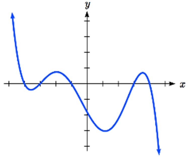
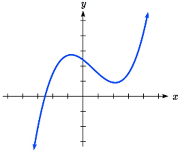
What is the least possible degree of the polynomial function shown in each graph?





Find the vertical and horizontal intercepts of each function.
$f(t)=2(t-1)(t+2)(t-3)$
$f(x)=3(x+1)(x-4)(x+5)$
$g(n)=-2(3n-1)(2n+1)$
$k(u)=-3(4-n)(4n+3)$
Graph each function using transformation techniques. Then identify the domain, range, intercepts, end behavior, and intervals of increasing or decreasing. Finally, identify any symmetry present.
$g(x)=(x-4)^2$
$h(x)=4-x^2$
$j(x)=-2x^2$
$k(x)=(-2x)^2$
$g(x)=(x-1)^3$
$h(x)=x^3-1$
$j(x)=- \frac{1}{2}x^{3}$
$k(x)=( - \frac{1}{2}x^{3})$
$g(x)=-(x+2)^2-1$
$h(x)=\left( \frac{1}{3}x - 1 \right)^{2}$
$j(x)=-(x+2)^3-1$
$h(x)=\left( \frac{1}{3}x - 1 \right)^{3}$