Section 1.7: Transformations
Describe how transformations affect the graphs of functions.
Throughout this book, we're going to want to be able to create quick sketches of functions. Before we get to specific functions, we'll investigate in general how graphs of functions can be moved, stretched, and flipped around the coordinate plane. Our motivational example for the results in this section is the graph of $y=f(x)$ below. While we could formulate an expression for $f(x)$ as a piecewise-defined function consisting of linear and constant parts, we wish to focus more on the geometry here. That being said, we do record some of the function values - the 'key points', or 'parent values', if you will - to track through each transformation.
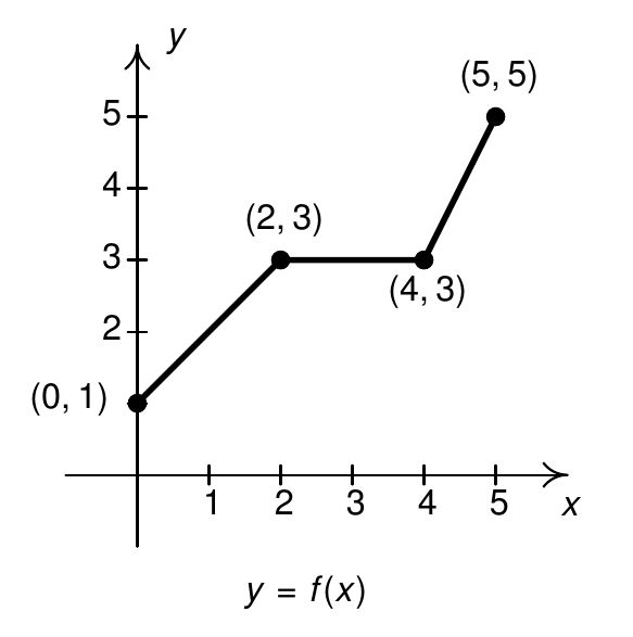
| $x$ | $y=f(x)$ |
|---|---|
| $0$ | $1$ |
| $2$ | $3$ |
| $4$ | $3$ |
| $5$ | $5$ |
| $(x,f(x))$ |
|---|
| $(0,1)$ |
| $(2,3)$ |
| $(4,3)$ |
| $(5,5)$ |
Vertical and Horizontal Shifts
Suppose we wished to graph $g(x)=f(x) + 2$. From a procedural point of view, we start with an input $x$ to the function $f$ and we obtain the output $f(x)$. The function $g$ takes the output $f(x)$ and adds $2$ to it. Using the sample values for $f$ from the table above we can create a table of values for $g$ below, hence generating points on the graph of $g$.
| $x$ | $f(x)\rightarrow$ | $g(x)=f(x) + 2$ | $(x, g(x))$ | |
|---|---|---|---|---|
| $0$ | $1$ | $1+2=3$ | $(0, 3)$ | |
| $2$ | $3$ | $3 + 2=5$ | $(2, 5)$ | |
| $4$ | $3$ | $3 + 2=5$ | $(4, 5)$ | |
| $5$ | $5$ | $5 + 2=7$ | $(5, 7)$ |
In general, if $(a,b)$ is on the graph of $y=f(x)$, then $f(a)=b$. Hence, $g(a)=f(a) +2=b+2$, so the point $(a,b+2)$ is on the graph of $g$. In other words, to obtain the graph of $g$, we add $2$ to the $y$-coordinate of each point on the graph of $f$.
To get a feel for what's happening here, you can adjust the slider labelled "d" in the following interactive demonstration. Consider the following: as d becomes larger, how does the graph change? What about as d becomes smaller (more negative)?
Made with Geogebra
Slide slider d to 2, and you'll see that geometrically, adding $2$ to the $y$-coordinate of a point moves the point $2$ units above its previous location. Adding $2$ to every $y$-coordinate on a graph en masse moves or 'shifts' the entire graph of $f$ up $2$ units. Notice that the graph retains the same basic shape as before, it is just $2$ units above its original location. In other words, we connect the four 'key points' we moved in the same manner in which they were connected before.
You'll note that the domain of $f$ and the domain of $g$ are the same, namely $[0,5]$, but that the range of $f$ is $[1,5]$ while the range of $g$ is $[3,7]$. In general, shifting a function vertically like this will leave the domain unchanged, but could very well affect the range.
You can perhaps imagine what would happen if we wanted to graph the function $j(x)=f(x) - 2$. Instead of adding $2$ to each of the $y$-coordinates on the graph of $f$, we'd be subtracting $2$. Geometrically, we would be moving the graph down $2$ units. We leave it to the reader to verify that the domain of $j$ is the same as $f$, but the range of $j$ is $[-1,3]$. In general, we have:
Vertical Shifts
Suppose $f$ is a function and $d$ is a real number.
To graph $F(x)=f(x) + d$, add $d$ to each of the $y$-coordinates of the points on the graph of $y=f(x)$.
NOTE: This results in a vertical shift up $d$ units if $d \gt 0$ or down $d$ units if $d \lt 0$.
Keeping with the graph of $y=f(x)$ above, suppose we wanted to graph $g(x)=f(x+2)$. In other words, we are looking to see what happens when we add $2$ to the input of the function. Let's try to generate a table of values of $g$ based on those we know for $f$. We quickly find that we run into some difficulties. For instance, when we substitute $x=4$ into the formula $g(x)=f(x+2)$, we are asked to find $f(4+2)=f(6)$ which doesn't exist because the domain of $f$ is only $[0,5]$. The same thing happens when we attempt to find $g(5)$.
| $x$ | $f(x)$ | $g(x)=f(x+2)$ | $(x,g(x))$ | |
|---|---|---|---|---|
| $0 $ | $1$ | $g(0)=f(0+2)=f(2)=3$ | $(0,3)$ | |
| $2 $ | $3 $ | $g(2)=f(2+2)=f(4)=3$ | $(2,3)$ | |
| $4 $ | $3$ | $g(4)=f(4+2)=f(6)=?$ | ? | |
| $5 $ | $5$ | $g(5)=f(5+2)=f(7)=? $ | ? |
What we need here is a new strategy. We know, for instance, $f(0)=1$. To determine the corresponding point on the graph of $g$, we need to figure out what value of $x$ we must substitute into $g(x)=f(x+2)$ so that the quantity $x+2$, works out to be $0$. Solving $x+2=0$ gives $x=-2$, and $g(-2)=f((-2)+2)=f(0)=1$ so $(-2,1)$ is on the graph of $g$.
Similarly, to use the fact that $f(2)=3$, we set $x+2=2$ to get $x=0$, which is the input we need for our $g$ function. Substituting gives $g(0)=f(0+2)=f(2)=3$. Continuing in this fashion, we produce the table below.
| $x $ | $ x+2 $ | $ g(x)=f(x+2) $ | $ (x, g(x))$ | |
|---|---|---|---|---|
| $-2 $ | $ 0 $ | $ g(-2)=f(-2+2)=f(0)=1 $ | $(-2, 1)$ | |
| $0 $ | $ 2 $ | $ g(0)=f(0+2)=f(2)=3 $ | $(0,3)$ | |
| $2 $ | $ 4 $ | $ g(2)=f(2+2)=f(4)=3 $ | $ (2,3)$ | |
| $3 $ | $ 5 $ | $ g(3)=f(3+2)=f(5)=5 $ | $ (3,5)$ |
In summary, the points $(0,1)$, $(2,3)$, $(4,3)$ and $(5,5)$ on the graph of $y=f(x)$ give rise to the points $(-2,1)$, $(0,3)$, $(2,3)$ and $(3,5)$ on the graph of $y=g(x)$, respectively.
In general, if $(a,b)$ is on the graph of $y=f(x)$, then $f(a)=b$. Solving $x+2=a$ gives $x=a-2$ so that $g(a-2)=f((a-2)+2)=f(a)=b$. As such, $(a-2,b)$ is on the graph of $y=g(x)$. The point $(a-2,b)$ is exactly $2$ units to the left of the point $(a,b)$ so the graph of $y=g(x)$ is obtained by shifting the graph $y=f(x)$ to the left $2$ units. To achieve this shift left, we subtract $c$ from our key $x$-values in the parent table. To get a feel for this, in the following demonstration, adjust the slider labelled c.
Made with Geogebra
Investigate what happens when $c$ is positive versus negative. It seems counterintuitive at first, but a positive $c$ value shifts the graph left while a negative $c$ value shifts the graph right!
Note that when we make $c=2$, while the ranges of $f$ and $g$ are the same, the domain of $g$ is $[-2,3]$ whereas the domain of $f$ is $[0,5]$. In general, when we shift the graph horizontally, the range will remain the same, but the domain could change. If we set out to graph $j(x)=f(x-2)$, we would find ourselves adding $2$ to all of the $x$ values of the points on the graph of $y=f(x)$ to effect a shift to the right $2$ units. Generalizing these notions produces the following result.
Horizontal Shifts
Suppose $f$ is a function and $c$ is a real number.
To graph $F(x)=f(x+c)$, subtract $c$ from each of the $x$-coordinates of the points on the graph of $y=f(x)$.
Note: This results in a horizontal shift right $c$ units if $c \lt 0$ or left $c$ units if $c \gt 0$.
These observations about vertical and horizontal shifts present a theme which will run common throughout the section: changes to the outputs from a function result in some kind of vertical change; changes to the inputs to a function result in some kind of horizontal change.
To regulate temperature in a green building, air flow vents near the roof open and close throughout the day to allow warm air to escape. The graph below shows the open vents V (in square feet) throughout the day, t in hours after midnight. During the summer, the facilities staff decides to try to better regulate temperature by increasing the amount of open vents by 20 square feet throughout the day. Sketch a graph of this new function.
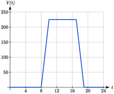
We can sketch a graph of this new function by adding 20 to each of the output values of the original function. This will have the effect of shifting the graph up.
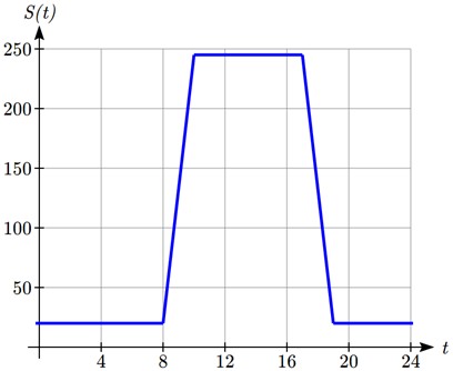
Notice that in the second graph, for each input value, the output value has increased by twenty, so if we call the new function $S(t)$, we could write $S(t)=V(t)+20$ .
Note that this notation tells us that for any value of t, S(t) can be found by evaluating the V function at the same input, then adding twenty to the result. This defines S as a transformation of the function V, in this case a vertical shift up 20 units.
Notice that with a vertical shift the input values stay the same and only the output values change.
In our next example, we're going to set up an organizational method for managing transformations in tables. We'll put our beginning "parent" $x$ and $y=f(x)$ values in the central column of the table. Then, we'll apply any $x$-transformations by adding columns onto the left side of the table (going out from the $x$ column), and we'll apply any $y$-transformations by adding columns onto the right side of the table (going out from the $y=f(x)$ column). That way, when we're done with the transformations, the outermost columns will form the coordinates for our transformed function.
A function $f(x)$ is given as a table below. Create a table for the function $g(x)=f(x)-3$
| $x$ | $f(x)$ |
|---|---|
| $2 $ | $ 1$ |
| $4 $ | $ 3 $ |
| $6 $ | $ 7 $ |
| $8 $ | $ 11$ |
The formula $g(x)=f(x)-3$ tells us that we can find the output values of the g function by subtracting 3 from the output values of the f function. For example, $$\begin{array}{ll} f(2)=1 & \text{is found from the given table}\\ g(x)=f(x)-3 & \text{is our given transformation}\\ g(2)=f(2)-3=1-3=-2& \end{array}$$ Subtracting 3 from each $f(x)$ value, we can complete a table of values for $g(x)$:
| $x$ | $f(x)\rightarrow$ | $g(x)=f(x)-3$ | $(x,g(x))$ | |
|---|---|---|---|---|
| $2 $ | $ 1$ | $g(2)=1-3=-2$ | $(2,-2)$ | |
| $4 $ | $ 3 $ | $g(4)=3-3=0$ | $(4,0)$ | |
| $6 $ | $ 7 $ | $g(6)=7-3=4$ | $(6,4)$ | |
| $8 $ | $ 11$ | $g(8)=11-3=8$ | $(8,8)$ |
The function $h(t)=-4.9t^2 +30t$ gives the height h of a ball (in meters) thrown upwards from the ground after t seconds. Suppose the ball was instead thrown from the top of a 10 meter building. Relate this new height function b(t) to h(t), then find a formula for b(t).
Returning to our building air flow example from the beginning of the section, suppose that in Fall, the facilities staff decides that the original venting plan starts too late, and they want to move the entire venting program to start two hours earlier. Sketch a graph of the new function.

In the new graph, which we can call $F(t)$, at each time, the air flow is the same as the original function $V(t)$ was two hours later. For example, in the original function $V$, the air flow starts to change at 8am, while for the function $F(t)$ the air flow starts to change at 6am. The comparable function values are $V(8)=F(6)$.
Notice also that the vents first opened to 220 sq. ft. at 10 a.m. under the original plan, while under the new plan the vents reach 220 sq. ft. at 8 a.m., so $V(10)=F(8)$ .
In both cases we see that since F(t) starts 2 hours sooner, the same output values are reached when, $F(t)=V(t+2)$.
Note that $V(t+2)$ had the effect of shifting the graph to the left.
A function f(x) is given as a table below. Create a table for the function $g(x)=f(x-3)$.
| $x $ | $ f(x)$ |
|---|---|
| $2 $ | $ 1 $ |
| $4 $ | $ 3 $ |
| $6 $ | $ 7$ |
| $8 $ | $ 11$ |
The formula $g(x)=f(x-3)$ tells us that the output values of g are the same as the output value of f with an input value three smaller. For example, we know that $f(2)=1$. To get the same output from the g function, we will need an input value that is 3 larger: We input a value that is three larger for g(x) because the function takes three away before evaluating the function f.
$$g(5)$$ $$=f(5-3)$$ $$=f(2)$$ $$=1$$So, to create our list of corresponding input values for the function $g$, we need to figure out what did we subtract that 3 from to get our list of inputs for $f(x)$? If we go in reverse, then we should add 3 to each of the input values for $f(x)$ to find what the inputs for $g$ need to be.
| $X=x+3$ | $\leftarrow x $ | $ f(x)$ |
|---|---|---|
| $X=2+3=5$ | $2 $ | $ 1 $ |
| $X=4+3=7$ | $4 $ | $ 3 $ |
| $X=6+3=9$ | $6 $ | $ 7$ |
| $X=8+3=11$ | $8 $ | $ 11$ |
| $x$ | $g(x)$ |
|---|---|
| $5$ | $1$ |
| $7$ | $3$ |
| $9$ | $7$ |
| $11$ | $11$ |
The result is that the function $g(x)$ has been shifted to the right by 3. Notice the output values for $g(x)$ remain the same as the output values for $f(x)$ in the chart, but the corresponding input values, $x$, have shifted to the right by 3: 2 shifted to 5, 4 shifted to 7, 6 shifted to 9 and 8 shifted to 11.
When thinking about horizontal and vertical shifts, it is good to keep in mind that vertical shifts are affecting the output values of the function, while horizontal shifts are affecting the input values of the function.
The function G(m) gives the number of gallons of gas required to drive m miles. Interpret $G(m)$ and $G(m+10)$.
$G(m)+10$ is adding 10 to the output, gallons. This is 10 gallons of gas more than is required to drive m miles. So, this is the gas required to drive m miles, plus another 10 gallons of gas.
$G(m+10)$ is adding 10 to the input, miles. This is the number of gallons of gas required to drive 10 miles more than m miles.
Reflections about the Coordinate Axes
We now turn our attention to reflections. You may know from algebra courses that to reflect a point $(x,y)$ across the $x$-axis, we replace $y$ with $-y$. If $(x,y)$ is on the graph of $f$, then $y=f(x)$, so replacing $y$ with $-y$ is the same as replacing $f(x)$ with $-f(x)$. Hence, the graph of $y=-f(x)$ is the graph of $f$ reflected across the $x$-axis. Similarly, the graph of $y=f(-x)$ is the graph of $y=f(x)$ reflected across the $y$-axis. To get a feel for this, in the following demonstration, adjust the sliders labelled a and b.
Made with Geogebra
Reflections
Suppose $f$ is a function.
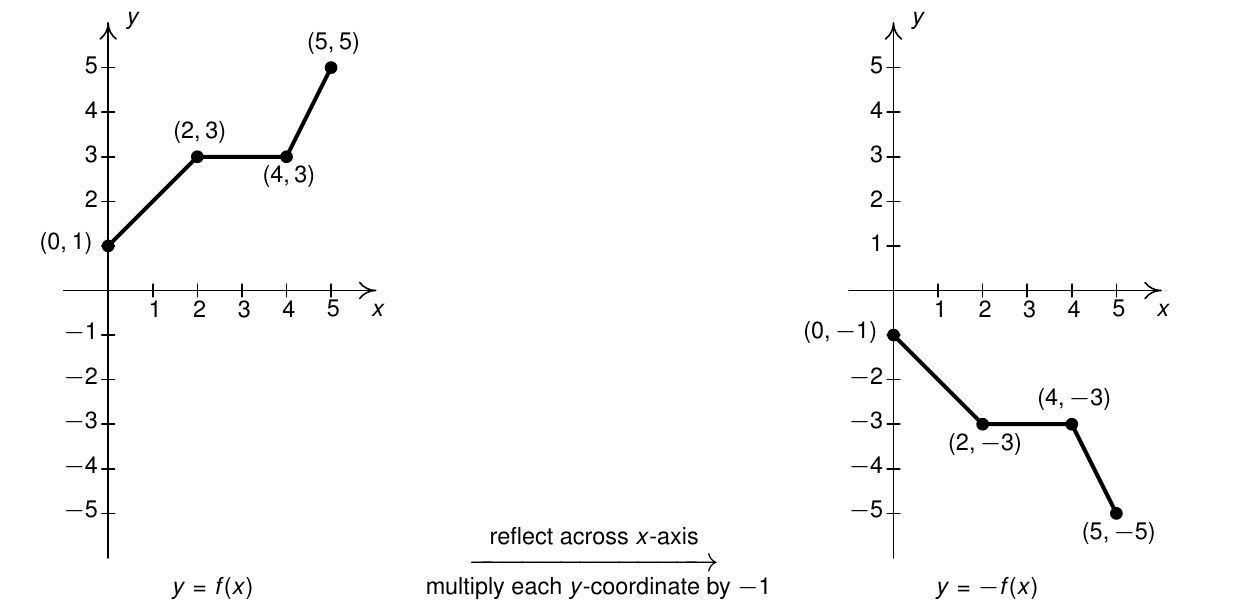
To graph $F(x)=-f(x)$, multiply each of the $y$-coordinates of the points on the graph of $y=f(x)$ by $-1$.
NOTE: This results in a reflection across the $x$-axis.
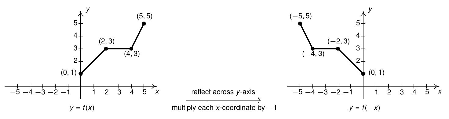
To graph $F(x)=f(-x)$, multiply each of the $x$-coordinates of the points on the graph of $y=f(x)$ by $-1$.
NOTE: This results in a reflection across the $y$-axis.
Using the language of inputs and outputs, we are saying that multiplying the outputs from a function by $-1$ reflects its graph across the horizontal axis, while multiplying the inputs to a function by $-1$ reflects the graph across the vertical axis.
Applying these ideas to the graph of $y=f(x)$ given at the beginning of the section, we can graph $y=-f(x)$ by reflecting the graph of $f$ about the $x$-axis.
| $x $ | $ y=f(x) $ | $ g(x)=-1\cdot y$ | $(x,g(x))$ | |
|---|---|---|---|---|
| $0 $ | $ 1 $ | $ -1 $ | $(0,-1)$ | |
| $2 $ | $ 3 $ | $ -3 $ | $(2,-3)$ | |
| $4 $ | $ 3 $ | $ -3 $ | $(4,-3)$ | |
| $5 $ | $ 5 $ | $ -5 $ | $(5,-5)$ |
By reflecting the graph of $f$ across the $y$-axis, we obtain the graph of $y=f(-x)$.
| $x $ | $ -x $ | $ g(x)=f(-x)$ | $(x,g(x))$ | |
|---|---|---|---|---|
| $0 $ | $ 0 $ | $ g(0)=f(-(-0))=f(0)=1 $ | $(0,1)$ | |
| $-2 $ | $ 2 $ | $ g(-2)=f(-(-2))=f(2)=3 $ | $(-2,3)$ | |
| $-4 $ | $ 4 $ | $ g(-4)=f(-(-4))=f(4)=3 $ | $(-4,3)$ | |
| $-5 $ | $ 5 $ | $ g(-5)=f(-(-5))=f(5)=5 $ | $(-5,5)$ |
A function $f(x)$ is given as a table below. Create a table for the function $g(x)=-f(x)$ and $h(x)=f(-x)$.
| $x $ | $ f(x)$ |
|---|---|
| $2 $ | $ 1 $ |
| $4 $ | $ 3 $ |
| $6 $ | $ 7$ |
| $8 $ | $ 11$ |
For $g(x)$, this is a vertical reflection, so the $x$ values stay the same and each output value will be the opposite of the original output value
| $x $ | $ y=f(x)\rightarrow $ | $ g(x)=-1\cdot y$ | $(x,g(x))$ | |
|---|---|---|---|---|
| $2 $ | $ 1 $ | $ -1$ | $(2,-1)$ | |
| $4 $ | $ 3 $ | $ -3$ | $(4,-3)$ | |
| $6 $ | $ 7 $ | $ -7$ | $(6,-7)$ | |
| $8 $ | $ 11 $ | $ -11$ | $(8,-11)$ |
For h(x), this is a horizontal reflection, and each input value will be the opposite of the original input value and the h(x) values stay the same as the f(x) values:
| $X=x\div -1 $ | $ x $ | $ f(x)$ | $(X,g(X))$ | |
|---|---|---|---|---|
| $-2 $ | $ 2 $ | $ 1$ | $(-2,1)$ | |
| $-4 $ | $ 4 $ | $ 3$ | $(-4,3)$ | |
| $-6 $ | $ 6 $ | $ 7$ | $(-6,7)$ | |
| $-8 $ | $ 8 $ | $ 11$ | $(-8,11)$ |
A common model for learning has an equation similar to $k(t)=-2^{-t}+1$, where k is the percentage of mastery that can be achieved after t practice sessions. This is a transformation of the function $f(t)=2^t$ shown here. Sketch a graph of $k(t)$.
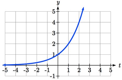
This equation combines three transformations into one equation.
We can sketch a graph by applying these transformations one at a time to the original function:

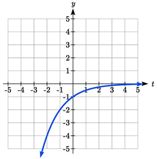
Then, after shifting up 1, we get the final graph.
$$k(t)=-f(-t)+1=-2^{-t}+1$$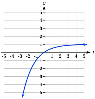
Note: As a model for learning, this function would be limited to a domain of $t\geq 0$, with corresponding range $[0,1)$.
Scalings
We now turn our attention to our last class of transformations: scalings. A thorough discussion of scalings can get complicated because they are not as straight-forward as the previous transformations. A quick review of what we've covered so far, namely vertical shifts, horizontal shifts and reflections, will show you why those transformations are known as rigid transformations.
Simply put, rigid transformations preserve the distances between points on the graph - only their position and orientation in the plane change. If, however, we wanted to make a new graph twice as tall as a given graph, or one-third as wide, we would be affecting the distance between points. These sorts of transformations are hence called non-rigid. As always, we motivate the general theory with an example.
Suppose we wish to graph the function $g(x) =2 f(x)$ where $f(x)$ is the function whose graph is given at the beginning of the section. From its graph, we can build a table of values for $g$ as before.
| $x $ | $ f(x) $ | $ g(x)=2f(x)$ |
|---|---|---|
| $0 $ | $ 1 $ | $ 2 $ |
| $2 $ | $ 3 $ | $ 6 $ |
| $4 $ | $ 3 $ | $ 6 $ |
| $5 $ | $ 5 $ | $ 10 $ |
| $(x, g(x))$ |
|---|
| $(0, 2)$ |
| $(2, 6)$ |
| $(4, 6)$ |
| $(5, 10)$ |
Graphing, we get:
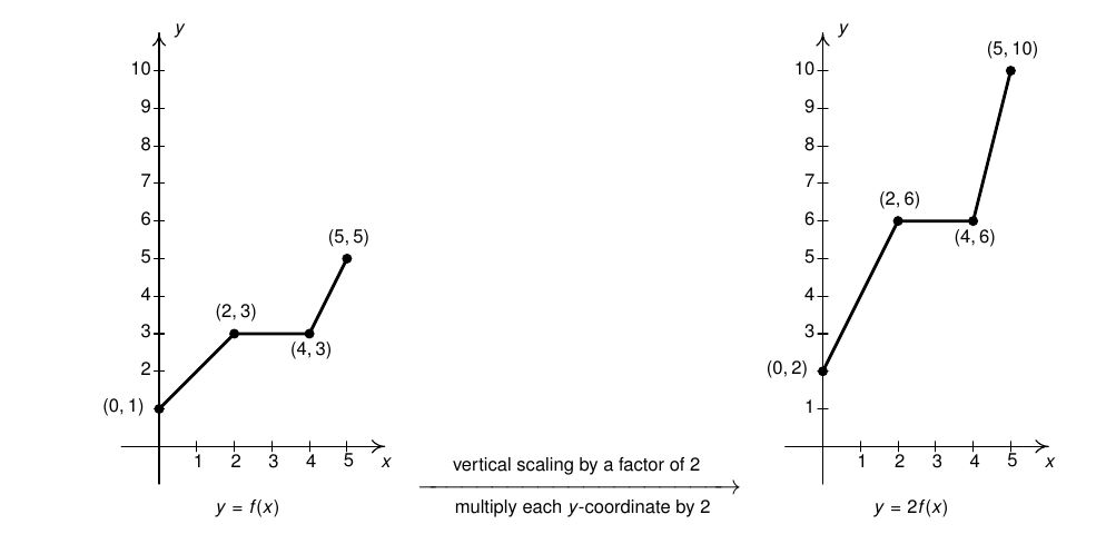
To get a feel for this, in the following demonstration, adjust the sliders labelled a.
Made with Geogebra
In general, if $(a,b)$ is on the graph of $f$, then $f(a)=b$ so that $g(a)=2 f(a)=2b$ puts $(a,2b)$ on the graph of $g$. In other words, to obtain the graph of $g$, we multiply all of the $y$-coordinates of the points on the graph of $f$ by $2$. Multiplying all of the $y$-coordinates of all of the points on the graph of $f$ by $2$ causes what is known as a 'vertical scaling by a factor of $2$', or a vertical stretch.
If we wish to graph $y=\frac{1}{2} f(x)$, we multiply the all of the $y$-coordinates of the points on the graph of $f$ by $\frac{1}{2}$. This creates a 'vertical scaling by a factor of $\frac{1}{2}$', or a vertical compression, as seen below.
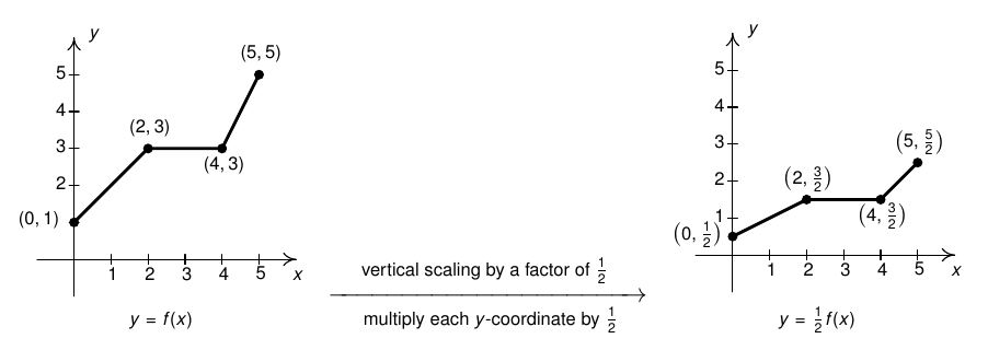
We generalize these results below.
Vertical Scalings.
Suppose $f$ is a function and $a>0$ is a real number.
To graph $F(x)=af(x)$, multiply each of the $y$-coordinates of the points on the graph of $y=f(x)$ by $a$.
- If $a \gt 1$, we say the graph of $f$ has undergone a vertical stretch by a factor of $a$.
- If $0 \lt a \lt 1$, we say the graph of $f$ has undergone a vertical shrink by a factor of $\frac{1}{a}$.
Referring to the graph of $f$ given at the beginning of this section, suppose we want to graph $g(x)=f(2x)$. In other words, we are looking to see what effect multiplying the inputs to $f$ by $2$ has on its graph. If we attempt to build a table directly, we quickly run into the same problem we had in our discussion leading up to our horizontal shifts, as seen in the following table.
| $x $ | $ f(x)$ | $ g(x)=f(2x) $ | $ (x, g(x)) $ |
|---|---|---|---|
| $0 $ | $ 1 $ | $ f(2 \cdot 0)=f(0)=1 $ | $(0, 1) $ |
| $2 $ | $ 3 $ | $ f(2\cdot2)=f(4)=3 $ | $(2,3) $ |
| $4 $ | $ 3 $ | $ f(2 \cdot 4)=f(8)=? $ | $ $ |
| $5 $ | $ 5 $ | $ f(2 \cdot 5)=f(10)=? $ | $ $ |
We solve this problem in the same way we solved this problem before. For example, if we want to determine the point on $g$ which corresponds to the point $(2,3)$ on the graph of $f$, we set $2x =2 $ so that $x=1$. Substituting $x=1$ into $g(x)$, we obtain $g(1)=f(2 \cdot 1)=f(2)=3$, so that $(1,3)$ is on the graph of $g$.
In general, if $(a,b)$ is on the graph of $f$, then $f(a)=b$. Hence $g\left(\frac{a}{2}\right)=f\left(2 \cdot \frac{a}{2}\right)=f(a)=b$ so that $\left(\frac{a}{2}, b\right)$ is on the graph of $g$. In other words, to graph $g$ we divide the $x$-coordinates of the points on the graph of $f$ by $2$. This results in a horizontal scaling by a factor of $\frac{1}{2}$.
| $X=\frac{x}2 $ | $ x $ | $ g(X)=f(2X)=f(x) $ | $ (X, g(X)) $ | |
| $0 $ | $ 0 $ | $ g(0)= f(2 \cdot 0)=f(0)=1 $ | $(0, 1) $ | |
| $1 $ | $ 2 $ | $ g(1)=f(2 \cdot 1)=f(2) =3 $ | $(1,3) $ | |
| $2 $ | $ 4 $ | $ g(2)=f(2 \cdot 2)=f(4)=3 $ | $ (2,3)$ | |
| $\frac{5}{2} $ | $ 5 $ | $ g\left(\frac{5}{2}\right)=f\left(2 \cdot \frac{5}{2} \right)=f(5)=5 $ | $\left(\frac{5}{2},5\right) $ |

To get a feel for this, in the following demonstration, adjust the slider labelled b.
Made with Geogebra
If, on the other hand, we wish to graph $y=f\left( \frac{1}{2} x\right)$, we end up multiplying the $x$-coordinates of the points on the graph of $f$ by $2$ which results in a horizontal scaling by a factor of $2$, as demonstrated below.
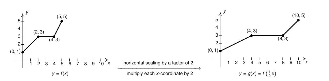
We generalize these results below.
Horizontal Scalings.
Suppose $f$ is a function and $b>0$ is a real number.
To graph $F(x)=f(bx)$, divide each of the $x$-coordinates of the points on the graph of $y=f(x)$ by $b$.
- If $0 \lt b \lt 1$, we say the graph of $f$ has undergone a horizontal stretch by a factor of $\frac{1}{b}$.
- If $b \gt 1$, we say the graph of $f$ has undergone a horizontal shrink by a factor of $b$.
A function P(t) models the growth of a population of fruit flies. The growth is shown in the graph. A scientist is comparing this to another population, Q, that grows the same way, but starts twice as large. Sketch a graph of this population.
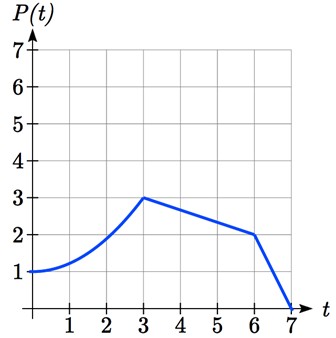
Since the population is always twice as large, the new population’s output values are always twice the original function output values. Graphically, this would look like the second graph shown.
Symbolically, $Q(t)=2P(t)$.
This means that for any input t, the value of the Q function is twice the value of the P function. Notice the effect on the graph is a vertical stretching of the graph, where every point doubles its distance from the horizontal axis. The input values, t, stay the same while the output values are twice as large as before.

A function $f(x)$ is given as a table below. Create a table for the function $g(x)=\frac12 f(x)$.
| $x $ | $ f(x)$ |
|---|---|
| $2 $ | $ 1 $ |
| $4 $ | $ 3$ |
| $6 $ | $ 7 $ |
| $8 $ | $ 11$ |
The formula $g(x)=\frac12 f(x)$ tells us that the output values of g are half of the output values of f with the same inputs. For example, we know that $f(4)=3$. Then $g(4)=\frac12 f(4)=\frac12(3)=\frac32$
| $x $ | $ y=f(x) $ | $ g(x) =\frac12\cdot y$ |
|---|---|---|
| $2 $ | $ 1 $ | $ 1\cdot \frac12=\frac12$ |
| $4 $ | $ 3 $ | $ 3\cdot \frac12=\frac32$ |
| $6 $ | $ 7 $ | $ 7\cdot \frac12=\frac72$ |
| $8 $ | $ 11 $ | $ 11\cdot \frac12=\frac{11}2$ |
| $(x, g(x))$ |
|---|
| $(2, \frac12)$ |
| $(4, \frac32)$ |
| $(6, \frac72)$ |
| $(8, \frac{11}2)$ |
The result is that the function g(x) has been compressed vertically by $\frac12$. Each output value has been cut in half, so the graph would now be half the original height.
Returning to the fruit fly population we looked at earlier, suppose the scientist is now comparing it to a population that progresses through its lifespan twice as fast as the original population. In other words, this new population, R, will progress in 1 hour the same amount the original population did in 2 hours, and in 2 hours, will progress as much as the original population did in 4 hours. Sketch a graph of this population.
Symbolically, we could write $$R(1)=P(2)$$ $$R(2)=P(4)$$
Graphing this, we have

Note the effect on the graph is a horizontal compression, where all input values are half their original distance from the vertical axis.
| $x $ | $ f(x)$ |
|---|---|
| $2 $ | $ 1$ |
| $4 $ | $ 3 $ |
| $6 $ | $ 7$ |
| $8 $ | $ 11$ |
The formula $g(x)=f(\frac12 x)$ tells us that the output values for $g$ are the same as the output values for the function $f$ at an input half the size. Notice that we don’t have enough information to determine since $g(2)=f(\frac12⋅2)=f(1)$, and we do not have a value for in our table. Our input values to g will need to be twice as large to get inputs for f that we can evaluate. For example, we can determine since $g(4)=f(\frac12⋅4)=f(2)=1$. Simply put, we'll multiply all our x-values by 2.
| $X=2\cdot x $ | $ \leftarrow x $ | $ f(x)$ |
|---|---|---|
| $4 $ | $ 2 $ | $ 1$ |
| $8 $ | $ 4 $ | $ 3$ |
| $12 $ | $ 6 $ | $ 7$ |
| $16 $ | $ 8 $ | $ 11$ |
| $(X, g(X))$ |
|---|
| $(4, 1)$ |
| $(8, 3)$ |
| $(12, 7)$ |
| $(16, 11)$ |
Since each input value has been doubled, the result is that the function $g(x)$ has been stretched horizontally by 2.
Two graphs are shown below. Relate the function $g(x)$ to $f(x)$.

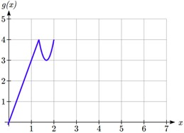
The graph of $g(x)$ looks like the graph of $f(x)$ horizontally compressed. Since $f(x)$ ends at $(6,4)$ and $g(x)$ ends at $(2,4)$ we can see that the $x$ values have been compressed by $1/3,$ because $6(1/3)=2.$ We might also notice that $g(2)=f(6)$, and $g(1)=f(3)$. Either way, we can describe this relationship as $g(x)=f(3x)$. This is a horizontal compression by $1/3.$
Transformations in Sequence
Now that we have studied three basic classes of transformations: shifts, reflections, and scalings, we present a result below which provides one algorithm to follow to transform the graph of $y=f(x)$ into the graph of $y=af(bx+c)+d$.
Transformations in Sequence.
Suppose $f$ is a function. If $a, b \neq 0$, then to graph $g(x)=a f(bx+c)+d$ start with the graph of $y=f(x)$ and follow the steps below.
- Subtract c from each of the $x$-coordinates of the points on the graph of $f$.
- Divide the $x$-coordinates of the points on the graph obtained in Step 1 by $b$.
- Multiply the $y$-coordinates of the points on the graph obtained in Step 2 by $a$.
- Add $d$ to each of the $y$-coordinates of the points on the graph obtained in Step 3.
NOTE: This results in a horizontal shift to the left if $c \lt 0$ or right if $c \gt 0$.
NOTE: This results in a horizontal scaling of factor $\frac1{b}$, but includes a reflection about the $y$-axis if $b \lt 0$.
NOTE: This results in a vertical scaling of factor $a$, but includes a reflection about the $x$-axis if $a \lt 0$.
NOTE: This results in a vertical shift up if $d \gt 0$ or down if $d \lt 0$.
A convenient way to remember this order is "C-BAD".
We should note that technically, the horizontal ($b$ and $c$) and vertical ($a$ and $d)$ transformations are independent of one another, so it doesn't matter whether we do the horizontal or the vertical first. For consistency's sake, though, we'll stick with the "C-BAD" order from here on out.
Given the table of values for the function $f(x)$ below, create a table of values for the function $g(x)=2f(3x)+1$.
| $x $ | $ y=f(x)$ |
|---|---|
| $6 $ | $ 10$ |
| $12 $ | $ 14$ |
| $18 $ | $ 15$ |
| $24 $ | $17$ |
Since $g(x)=2f(3x)+1$, we have $a=2$, $b=3$, and $d=1$. Technically, $c=0$, so we'll skip that transformation.
We'll put our original, parent values in the center of our table and work outward from there in C-BAD order.
| $X=\frac13 x $ | $ \leftarrow x $ | $ y=f(x) \rightarrow $ | $ 2\cdot y \rightarrow $ | $ 2\cdot y +1$ |
|---|---|---|---|---|
| $2 $ | $ 6 $ | $ 10 $ | $ 20 $ | $ 21$ |
| $4 $ | $ 12 $ | $ 14 $ | $ 28 $ | $ 29$ |
| $6 $ | $ 18 $ | $ 15 $ | $ 30 $ | $ 31$ |
| $8 $ | $ 24 $ | $ 17 $ | $ 34 $ | $ 35$ |
The outer columns then form our final, transformed function:
| $X $ | $ g(X)$ |
| $2 $ | $ 21$ |
| $4 $ | $ 29$ |
| $6 $ | $ 31$ |
| $8 $ | $ 35$ |

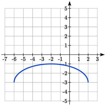
We'll start by identifying $a$, $b$, $c$, and $d$. Here we have $b=\frac12$, $c=1$, and $d=-3$. Technically $a=1$, but that won't reflect or stretch the graph, so we'll ignore it.
We can follow our same C-BAD process if we pick out a few points on our graph to use as the parent function. We'll use $(-2, 0)$, $(0, 2)$, and $(2, 0)$. We'll put those parent values in the center of our table, and work outwards from there in C-BAD order.
First, subtract 1 from the $x$-values (a shift to the left). Then divide the new $x$-values by $\frac12$ (which is the same as multiplying by the reciprocal, 2, a horizontal stretch). Finally, we'll subtract 3 from the $y$-values (a vertical shift down).
| $X=(x-1)\cdot 2 $ | $\leftarrow x - 1 $ | $\leftarrow x $ | $ y=f(x) \rightarrow $ | $ y - 3$ |
|---|---|---|---|---|
| $-6 $ | $ -3 $ | $ -2 $ | $ 0 $ | $ -3$ |
| $-2 $ | $ -1 $ | $ 0 $ | $ 2 $ | $ -1$ |
| $2 $ | $ 1 $ | $ 2 $ | $ 0 $ | $ -3$ |
So, our final table for $k(x)$, taken from the outer columns of our transformation, is:
| $X $ | $ k(X)$ |
|---|---|
| $-6 $ | $ -3 $ |
| $-2 $ | $ -1$ |
| $2 $ | $ -3$ |
We can now plot those points and connect them with the same semicircular shape that we saw in the parent function:
Given the original function $f(x)$ and transformed function $g(x)$ pictured below, find a, b, c, and d so that $g(x)=a f(b x + c) + d$.
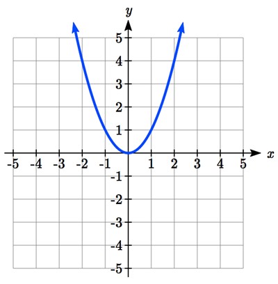
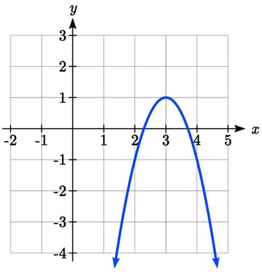
The original function has been flipped over the x axis, some kind of stretch or compression has occurred, and we can see a shift to the right 3 units and a shift up 1 unit.
In total there are four operations:
- Vertical reflection, requiring a negative sign outside the function
- Vertical Stretch or Horizontal Compression*
- Horizontal Shift Right 3 units, which tells us to put x-3 on the inside of the function
- Vertical Shift up 1 unit, telling us to add 1 on the outside of the function
* It is unclear from the graph whether it is showing a vertical stretch or a horizontal compression. For this shape, it turns out we could represent it either way, so we’ll use a vertical stretch. You may be able to determine the vertical stretch by observation.
By observation, the basic function has a vertex at (0, 0) and symmetrical points at $(1, 1)$ and $(-1, 1).$ These points are one unit up and one unit over from the vertex. The new points on the transformed graph are one unit away horizontally but 2 units away vertically. They have been stretched vertically by two.
So, a vertical stretch of 2 means $a=2$. A reflection across the $x$-axis furthermore means this $a$ value should be negative. A move right means that our $c$ value needs to be negative 3. A move up 1 means $d=1$. Therefore $$g(x)=-2f(x-3)+1$$
Important Topics of this Section
Transformations
Vertical Shift (up & down)
Horizontal Shifts (left & right)
Reflections over the vertical & horizontal axis
Vertical Stretches & Compressions
Horizontal Stretches & Compressions
Combinations of Transformation
Section 1.7 Exercises
Conceptual Questions
- In the structure $g(x)=a f(bx+c)+d,$ what do each of the constants $a, b, c,$ and $d$ do?
- In the structure $g(x)=af(bx+c)+d,$ what is special about the way that $b$ and $c$ work, versus $a$ and $d?$
- In the structure $g(x)=af(bx+c)+d),$ what values affect the $x$’s? What values affect the $y$’s?
Practice Problems
Describe how each function is a transformation of the original function $f(x)$
- $f(x-49)$
- $f(x+43)$
- $f(x+3)$
- $f(x-4)$
- $f(x)+5$
- $-f(x)$
- $f(5x)$
- $3f(-x)$
- $6f(x)$
- $f\left(\frac15 x\right)$
- $f(x)+8$
- $f(x)-2$
- $f(x)-7$
- $f(x-2)+3$
- $f(x+4)-1$
- $4f(x)$
- $f\left(\frac13 x\right)$
- $f(-x)$
- $f(2x)$
- $-f(3x)$
Shift right 49
Shift left 3
Shift up 5
Horizontally compress by 1/5
Vertically stretch by 6
Shift up 8
Shift down 7
Shift left 4 and down 1
Horizontal stretch by 3
Horizontal compress by ½
- Write a formula for $f(x)$ shifted up 1 unit and left 2 units.
- Write a formula for $f(x)$ shifted down 3 units and right 1 unit.
- Write a formula for $f(x)$ shifted down 4 units and right 3 units.
- Write a formula for $f(x)$ shifted up 2 units and left 4 units.
- Write a formula for $f(x)$ reflected about the $x$-axis.
- Write a formula for $f(x)$ reflected about the $y$-axis.
- Write a formula for $f(x)$ reflected over the y axis and horizontally compressed by a factor of $\frac14$.
- Write a formula for $f(x)$ reflected over the x axis and horizontally stretched by a factor of 2.
- Write a formula for $f(x)$ vertically compressed by a factor of $\frac13$, then shifted to the left 2 units and down 3 units.
- Write a formula for $f(x)$ vertically stretched by a factor of 8, then shifted to the right 4 units and up 2 units.
- Write a formula for $f(x)$, shifted to the right 5 units, horizontally compressed by a factor of $\frac12$, and shifted up 1 unit.
- Write a formula for $f(x)$ shifted to the left 4 units, horizontally stretched by a factor of 3, then shifted down 3 units.
$f(x+2)+1$
$f(x−3)-4$
$-f(x)$
$f(−4x)$
$\frac{1}{3}f(x + 2) - 3$
$f(2x−5)+1$
- Tables of values for $f(x), g(x)$, and $h(x)$ are given below. Write $g(x)$ and $h(x)$ as transformations of $f(x)$.
$x $ $ f(x)$ $-2 $ $ -2$ $-1 $ $ -1 $ $0 $ $ -3 $ $1 $ $ 1 $ $2 $ $ 2$ $x $ $ g(x)$ $-1 $ $ -2$ $0 $ $ -1 $ $1 $ $ -3 $ $2 $ $ 1 $ $3 $ $ 2$ $x $ $ h(x)$ $-2 $ $ -1$ $-1 $ $ 0 $ $0 $ $ -2 $ $1 $ $ 2 $ $2 $ $ 3$ $g(x) = f(x−1)$; $h(x) = f(x)+1$
- Tables of values for $f(x), g(x)$, and $h(x)$ are given below. Write $g(x)$ and $h(x)$ as transformations of $f(x)$.
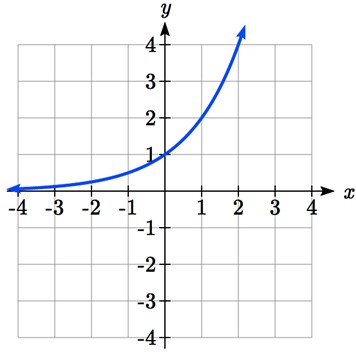
$x $ $ f(x)$ $-2 $ $ -1$ $-1 $ $ -3 $ $0 $ $ 4$ $1 $ $ 2 $ $2 $ $ 1$ $x $ $ g(x)$ $-3 $ $ -1$ $-2 $ $ -3 $ $-1 $ $ 4$ $0 $ $ 2 $ $1 $ $ 1$ $x $ $ h(x)$ $-2 $ $ -2$ $-1 $ $ -4 $ $0 $ $ 3$ $1 $ $ 1 $ $2 $ $ 0$ - The graph of $f(x)=2^x$ is shown. Sketch a graph of each transformation of $f(x)$. Then describe the domain and range of each transformed graph.
- $g(x)=f(x) + 1$
- $h(x)=f(x) - 3$
- $w(x)=f(x-1)$
- $q(x)=f(x+3)$
- $r(x)=-f(x)+1$
- $j(x)=f(-x)$
(a)
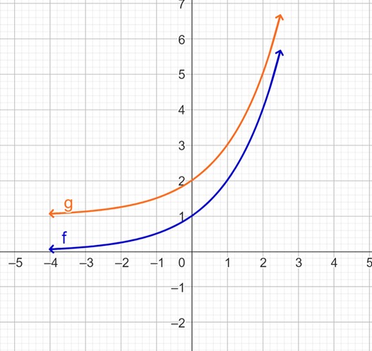
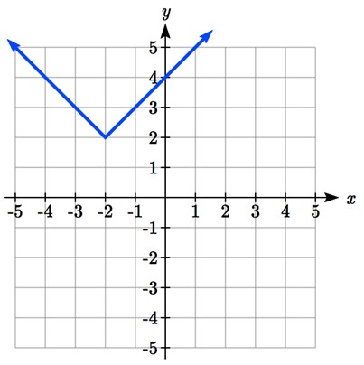
- The graph of $f(x)=|x|$ is shown. Sketch a graph of each transformation of $f(x)$. Then, describe the interval(s) on which the function is increasing or decreasing.

- $g(x)=f(x+1)-3$
- $h(x)=f(x-1)+4$
- $k(x)=f(x-2)-1$
- $m(x)=3+f(x+2)$
- $p(x)=-2f(x-4)+3$
- $n(x)=\frac13 f(x-2)$
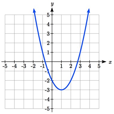
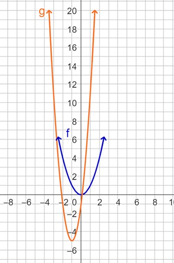
- The graph of $f(x)=x^2$ is shown. Sketch a graph of each transformation of $f(x)$. Then, describe the interval(s) on which the function is increasing or decreasing. Finally, determine the interval(s) on which the function is concave up and concave down.
- $g(x)=4f(x+1)-5$
- $h(x)=5f(x+3)-2$
- $p(x)=f\left(\frac13 x \right) -3$
(a)
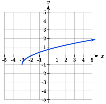
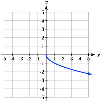
- The graph of $f(x)= \sqrt{x}$ is shown. Sketch a graph of each transformation of $f(x)$. Then, describe the interval(s) on which the function is increasing or decreasing. Finally, determine the interval(s) on which the function is concave up and concave down.
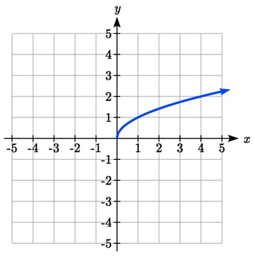
- $k(x)=-3f(x)-1$
- $a(x)=f(-x+4)$
-
$$f(x)$$
-
$$f(x)$$
-
$$f(x)$$
-
$$f(x)$$
-
$$f(x)$$
-
$$f(x)$$
-
$$f(x)$$
-
$$f(x)$$

-
$$f(x)$$
-
$$f(x)$$
$g(x) = f(x−3)-2$
$g(x) = f(x+3)-1$
$g(x) = -f(x)$
$g(x) = -f(x+1)+2$
$g(x) = f(−x)+1$
(b) 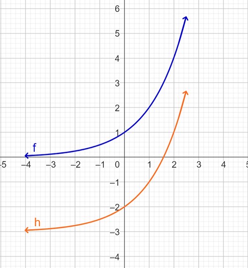
(c) 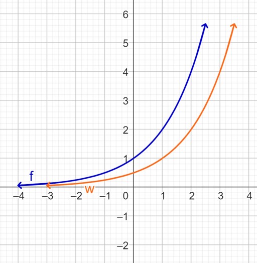
(d) 
(e) 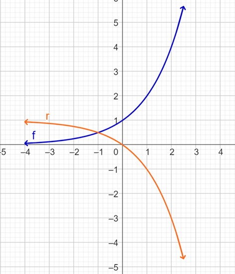
(f) 
(b) 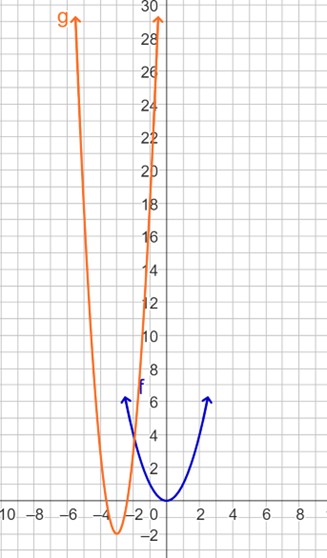
(c) 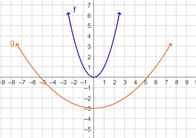
Given each graph of $f(x)$ and $g(x)$ below, find $a$, $b$, $c$, and $d$ such that $g(x)=af(bx+c)+d$.