Lab Six: Remote Sensing - Using Landsat Imagery and NDVI to Distinguish Vegetation near Pueblo, Colorado
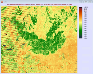
Black Forest area, Colorado. Thanks to Landsat, differences in vegetation are clear.
Lab Six Goals
To explore basics of remote sensing (RS) and image processing. Students will:
- download Landsat imagery from the USGS Global Visualization Viewer (GLOVIS)
- explore some basic functions of IDRISI TerrSet, a robust and fairly common remote sensing software (IDRISI TerrSet)
- work with multispectral satellite data (Landsat Band 3 (red) and Band 4 (near-infrared)) (Landsat)
- ingest the concept of a normalized difference vegetation index (NDVI) applied to a semi-arid, mixed-use climate
Lab Overview
Students download USGS Landsat imagery of the southeast Colorado region, extract (unzip) the compressed files, import and convert the files from .tif to.rst format, generate a final NDVI image, and adjust display properties to distinguish irrigated vegetation from non-irrigated vegetation. Like previous labs, the images posted to the lab web page contain a descriptive caption that interprets the scene. Students are responsible for answering the questions below in red.
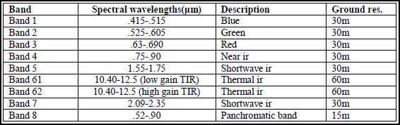 |
Table 1: Landsat band specifications |
Due 5:00 p.m., Sunday, Apr. 14
Tools
- IDRISI TerrSet Geospatial Monitoring and Modeling System
- Expression Web 4
- Filezilla
- A web browser
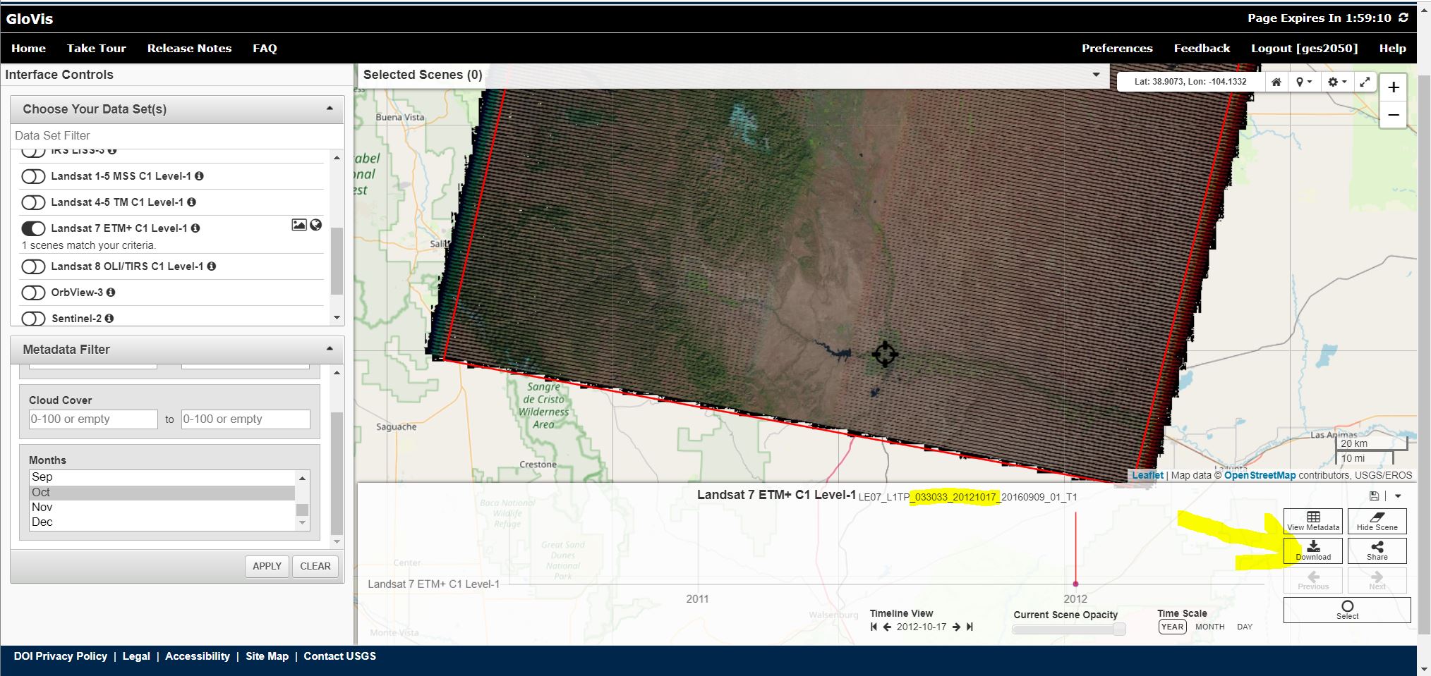
Part One: Download October 17, 2012 Landsat Scene (path 33, row 33) from USGS GLOVIS Website
- Go to http://glovis.usgs.gov/ Launch Glovis. This is the website from which you will download Landsat imagery.
- The goal in Part One is to download a "Landsat 7 Enhanced Thematic Mapper Plus (ETM+)" scene (multispectrail imagery) that covers a 183 x 170 km region of southeast Colorado, including Pueblo and Colorado Springs, collected precisely on October 17, 2012.
- The first step is to make sure the GLOVIS site is set up to deliver the correct product (Landsat 7 ETM+ from 2012):
- To download the data set:
- Click the little 'Download' icon in the box, then click 'DOWNLOAD' for the 'Level-1 GeoTIFF Data Product (231.05 MB)'
- 'Save As' the zipped file to your Z drive, specifically, in your Lab Six folder. Hint: why not create a 'working' or 'data' folder in your lab six folder?
- Next, you need to unzip the files: Right-click on the file to unzip (unzip into the same folder).
- After the files have been unzipped / extracted, I suggest that you delete the original zipped (.tar) file simply to save storage space on your z drive.
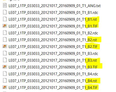
- Notice the different bands (B1, B2, B3, etc.))
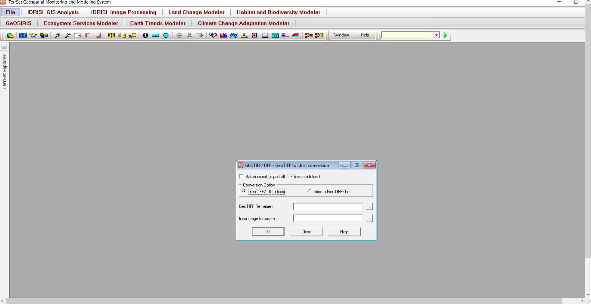
Part Two: Convert Images from .TIF to .RST in IDRISI TerrSet
- Before you can work with the Landsat (US Government) scenes (images) in TerrSet, you MUST perform a file conversion -- from .TIF to .RST
- Open IDRISI TerrSet software -- Close the "Tip" window
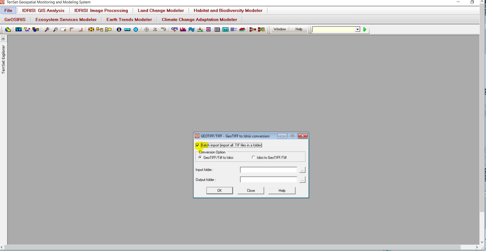
- Go: File > Import > Government / Data Provider Formats > GEOTIFF/TIF. You'll see a screen like this.
- Check the 'geoTIFF/Tiff to Idrisi' button.
- Turn on (check) the radio button 'Batch import (import all .TIF files in a folder)
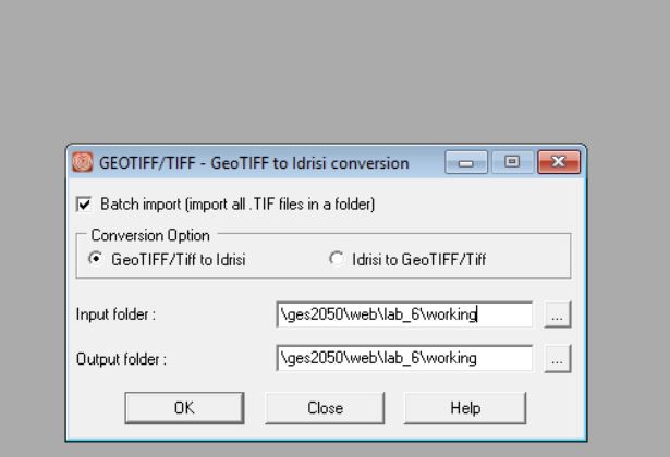
- Using the the 'pick list' (the little icons with three dots along the bottom), browse to the 'Input folder' and 'Output folder 'like this (this is the FOLDER in which your LANDSAT imagery are stored on your Z drive (a directory in your lab six folder somewhere).
- CLICK 'OK' ONE TIME AND WAIT A FULL ONE OR TWO MINUTES.
- Your files will convert from .TIF to .rst. Look in your lab six folder to verify - you will now see both .TIF and .rst
- Close the 'GEOTIFF/TIFF - GeoTIFF to Idrisi conversion' window.
Part Three: Use IDRISI TerrSet 'VEGINDEX' to Create NDVI Image
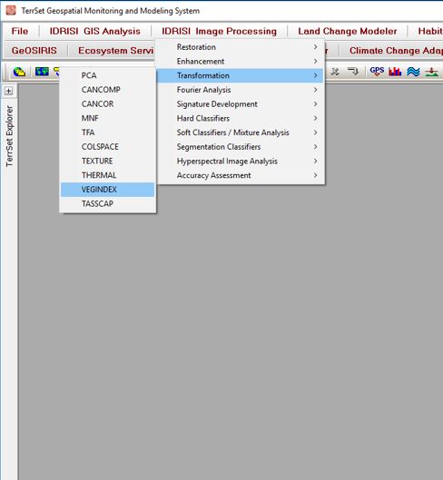
- TerrSet offers a built-in program called “VEGINDEX” that calculates ~20 variations of vegetation indices. You will practice with a very common index, the NDVI (we talked about this in class).
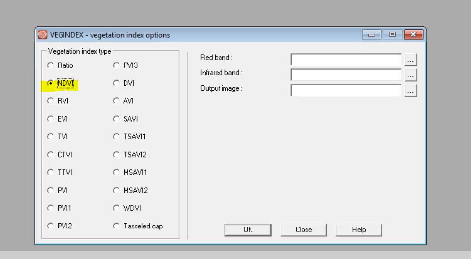
- Start VEGINDEX from the main menu (Go: IDRISI Image Processing > Transformation > VEGINDEX)
- Select the radio button for NDVI (NOT the default, which is probably 'Ratio').
- You will be using only two bands for NDVI: band 3 (red) and band 4 (near IR). SEE TABLE 1 above for specifications.
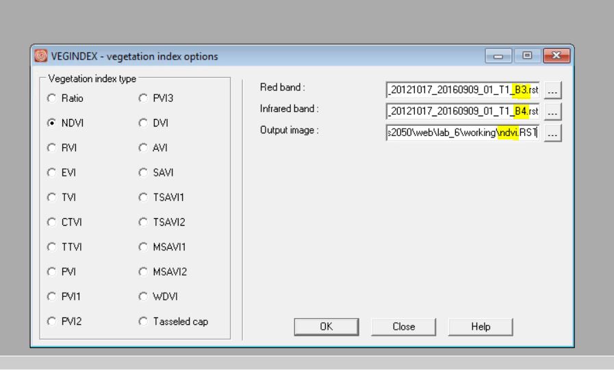
- You will again have to use the 'pick list' (the little icons with three dots along the bottom) to browse to the correct bands (these are stored on your Z drive in your lab six folder)
- Knowing that red is Landsat band 3 and near-IR is Landsat band 4, fill in the inputs like this. BE SURE to give your 'output image' a file name like ndvi and save to your lab six working directory.
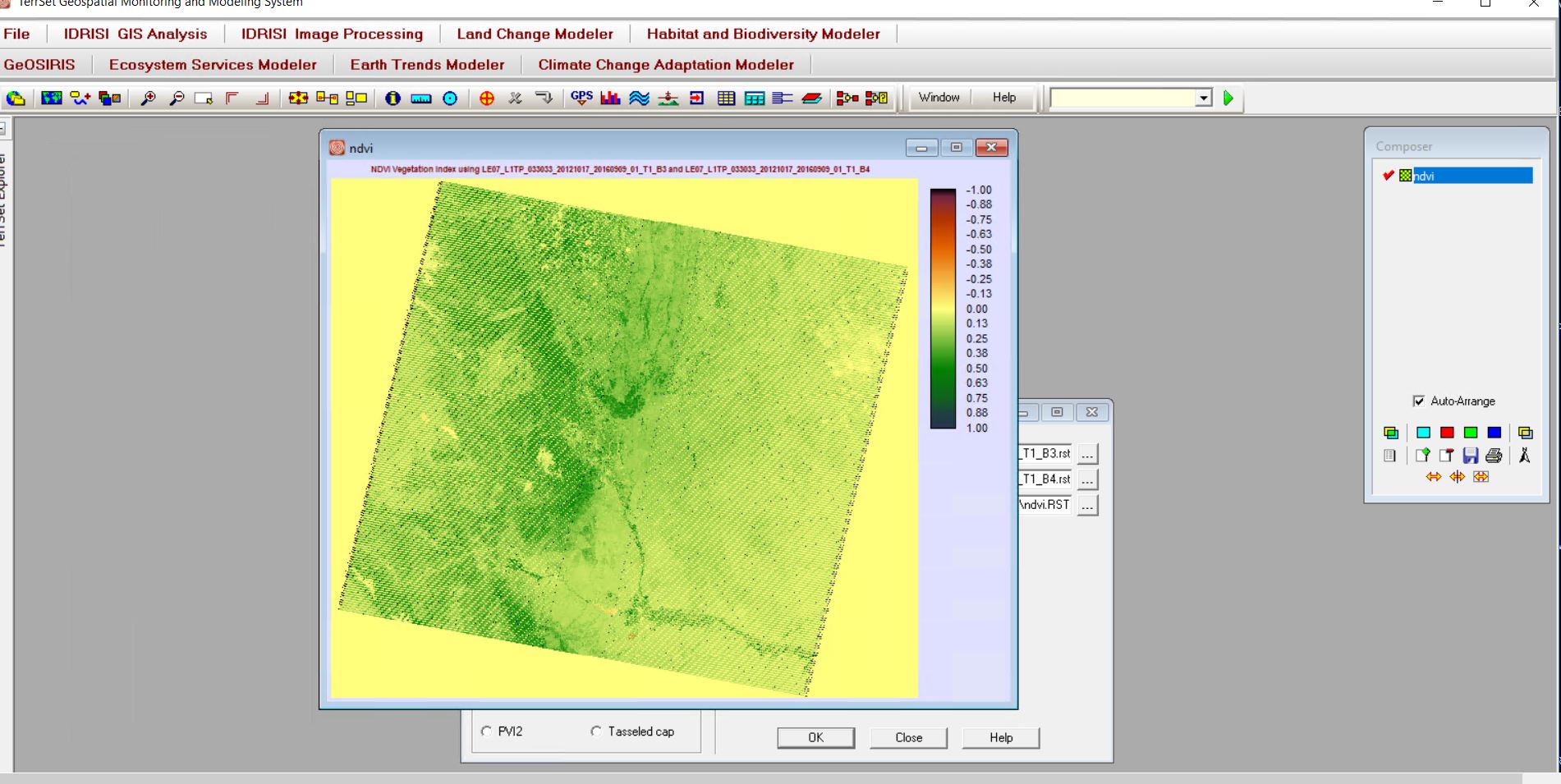
- Click OK to generate and display the image. This image looks okay but the colors are all very similar -- and not using the full range available in the color ramp! Let's fix that in Part Four.
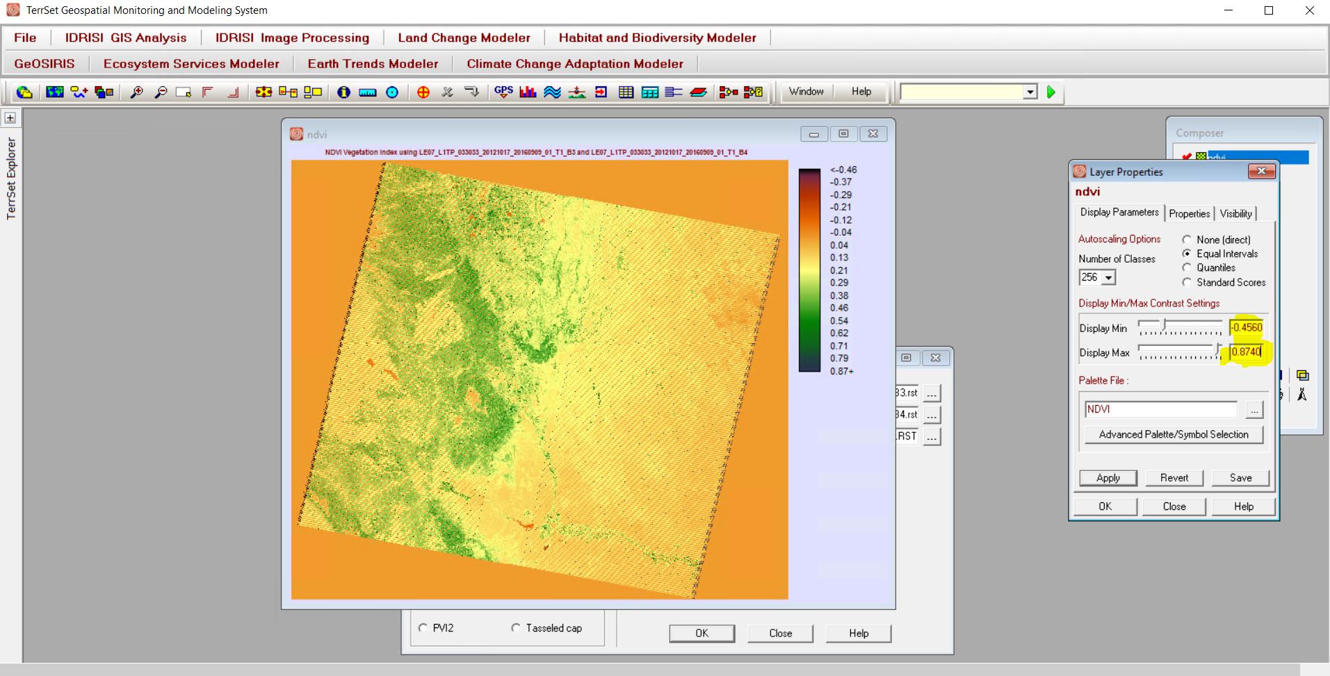
Part Four: Adjust Display Properties So Digital Number (DN) Range Falls between +1 (Green, Healthy Vegetation) and -1 (No Vegetation)
- You need to maximize the available range of (false) colors to help us better distinguish vegetation greeness.
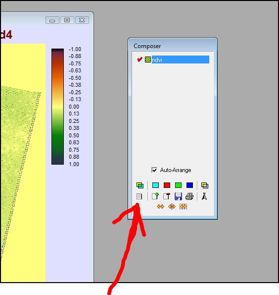
- In the little 'Composer window' in TerrSet, click on the Layer properties button.
- Experiment with the sliders -- after experimenting, set the values in the 'Display Min' text box to -0.456 and change the values in the 'Display Max' text box to 0.874. Again, do this to MAXIMIZE how you SEE variation -- to my brain and to my vision, these numbers (-0.456 and 0.874) seem to work well.
- Click 'Apply' and then 'Save'
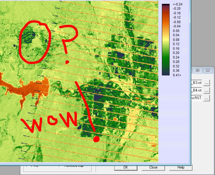
- Using the 'Zoom' tool, zoom in to the Pueblo Reservoir area. Adjust the sliders to further maximize water from vegetation from urban (?). Wow!
- Feeling bold? As an option, start over with a different month or worldly location (paying attention to cloud cover). Landsat is good science indeed. Can you imagine the possibilities?
What I Grade
- Your final NDVI scene created in Part Four (one .jpg screenshot from TerrSet) with caption of a zoomed-in section of your choice
- The answers to the following questions (include the set of questions on your Lab Six web page):
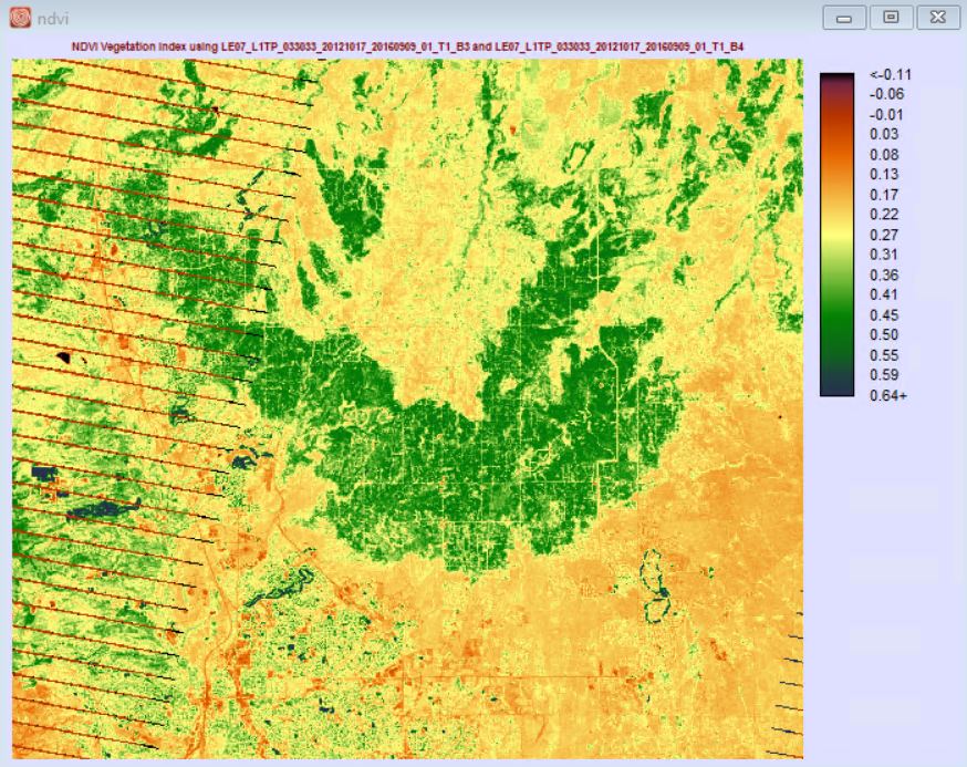
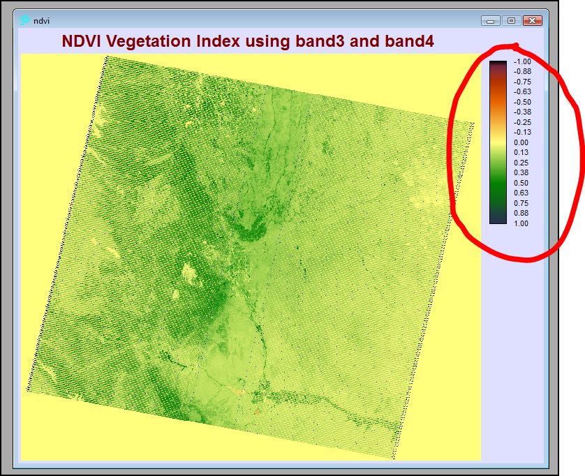
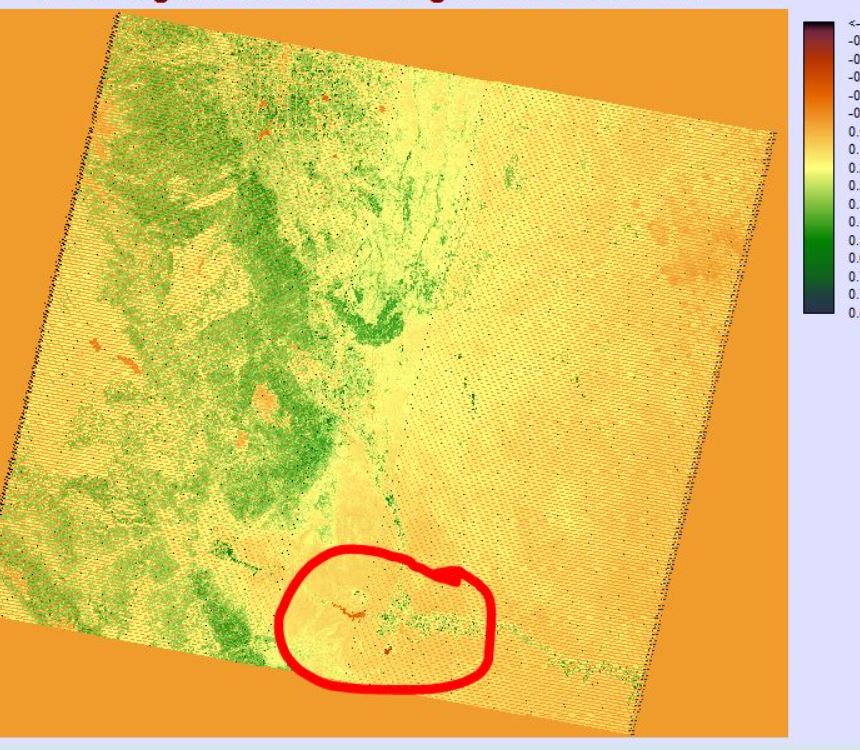
- Why do you see gaps in data (slices of missing imagery) in the Landsat 7 ETM+ scenes, as seen in the NDVI image below? (HINT: read this NASA article)
- Why is it vital to trees that i) leaves absorb visible light and ii) scatter (not use) near-infrared radiation? Use reputable online sources to help construct your answer (and provide the source web site(s) credit by providing link(s)). Note that this is a two-part question.
- The radiometric resolution of Landsat 7 ETM+ imagery, including Band 3 (red) and Band 4 (near IR), is 256. What are the VALUES for the other three resolutions (spatial, spectral, and temporal) for Landsat 7 ETM+ Band 3 and Band 4?
- Provide and summarize THREE examples of how Landsat has been used to solve real-world problems (other than problems associated with vegetation). This will take some outside research on your part. You do not need to provide source website like you did with Question #2 above).
- Example 1:
- Example 2:
- Example 3:
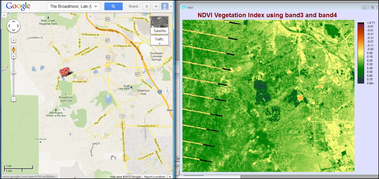
A fun exercise (NOTHING GRADED BELOW - Just an FYI): Compare image at left (Google Maps) to image at right (NDVI) to see just how NDVI works.
I picked a local place - S. Tejon / S. Nevada / Broadmoor area (reservoirs, roads, golf courses, irrigated lawns, mature decidous trees) to help you interpret Landsat / IDRISI NDVI results.
Scene from Oct. 17, 2012 imagery. To ponder: I wonder if you can detect hail damage from the 'Cheyenne Mouuntain Zoo Hailstorm' of Aug. 6, 2018?
