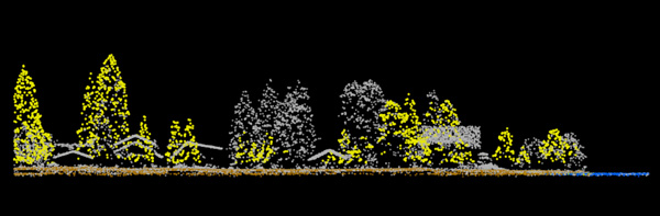
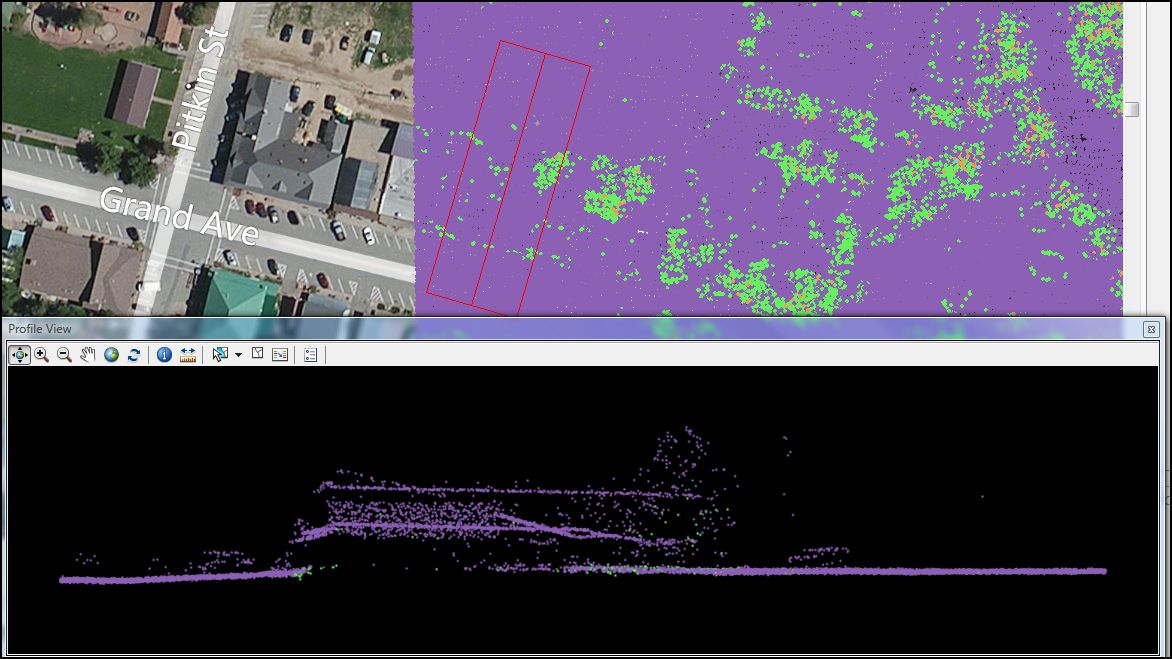
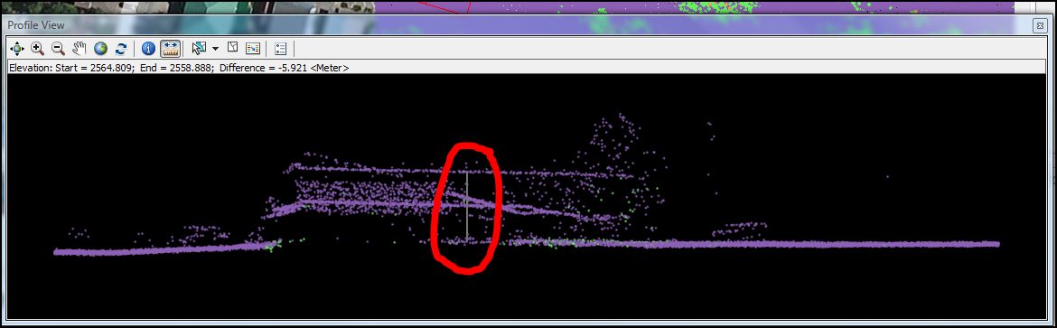
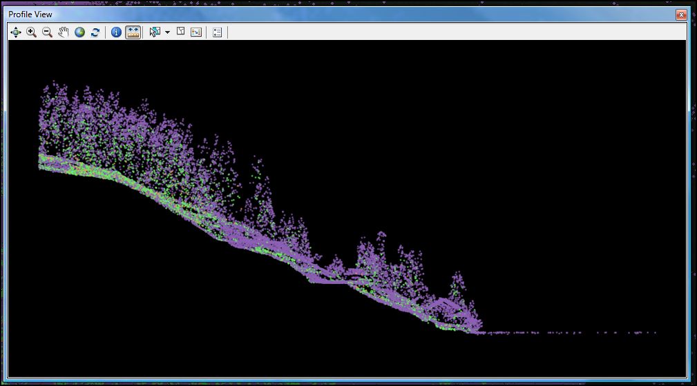
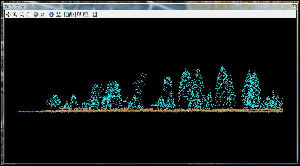
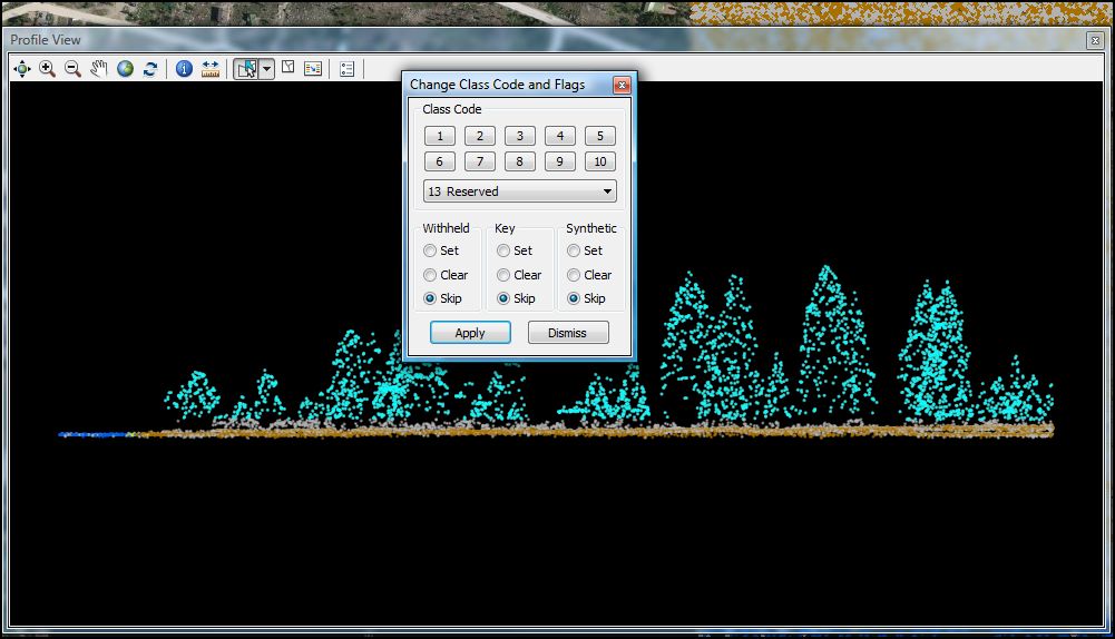
Several classes of airborne lidar data along a cabin-lined stream, Grand Lake, Colorado.
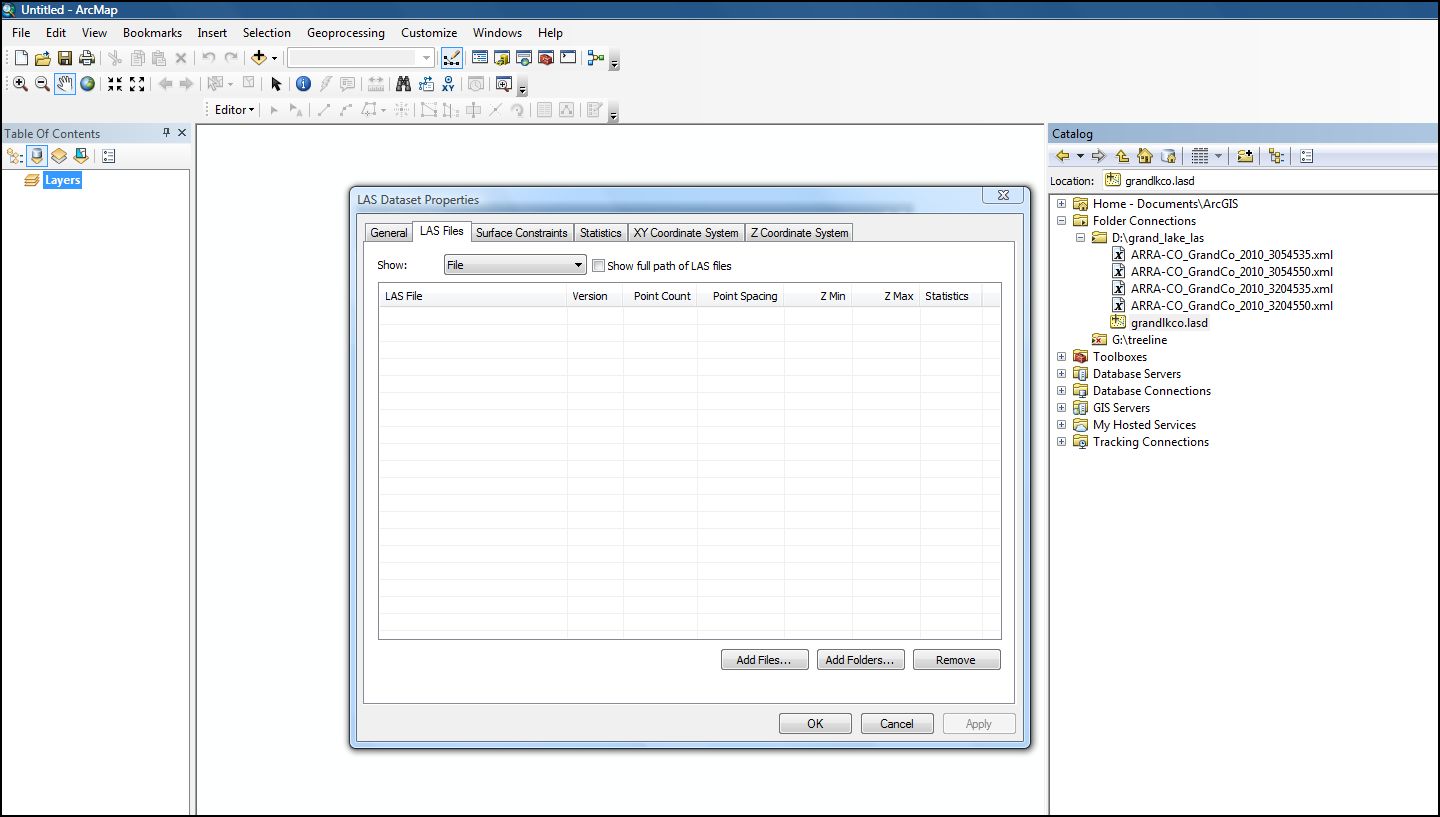
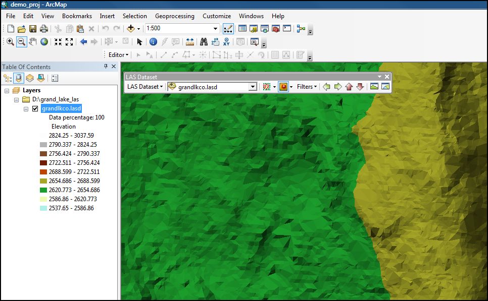
Working with USGS airborne lidar .las files (from USGS' CLICK) in ArcMap 10.1
|
Several classes of airborne lidar data along a cabin-lined stream, Grand Lake, Colorado.
|
Goal:
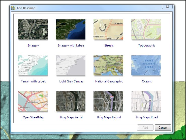
Software:
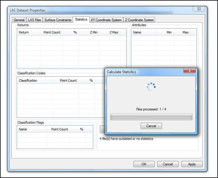
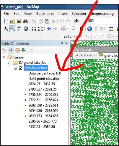
Steps:
NOTE: Much of the workflow outlined in this tutorial was borrowed from here and here.
Problems? Ask Brandon: bvogt @ uccs.edu