Interpolation of Airborne and Terrestrial Lidar Data

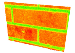
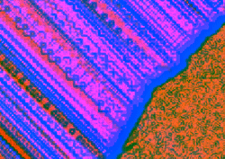
A dense point cloud of a brick wall surface	Interpolation edge streamers - an artifact of what?

• to work with airborne and terrestrial lidar datasets
• to import x, y, z text files (*.txt) into a GIS project
• to interpolate point data (vector to raster)
• to view 3D point clouds in ArcScene

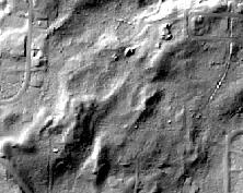
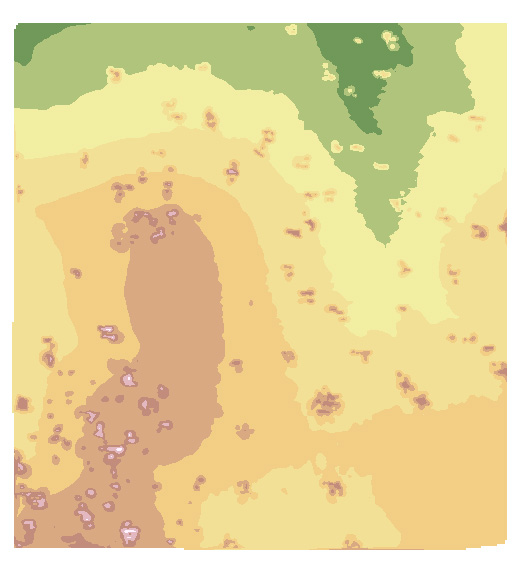
Interpolated first returns from airborne lidar of a section of W. Denver

Tools

• Notepad
• Pre-processed airborne and terrestrial lidar point data
• ArcMap with Spatial Analyst Extension
• ArcScene
• Expression Web 4
• Filezilla
• a web browser

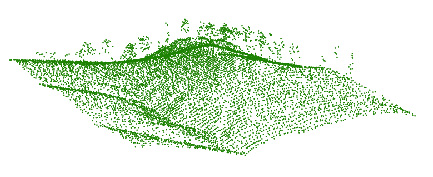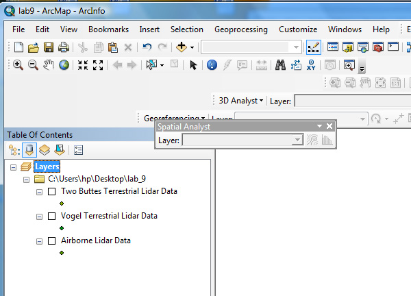
Raw airborne lidar data in Shapefile format. Do you see the trees?

Introduction

This exercise focuses on data interpolation. That is, creating rasters from points by filling data-free spaces as best possible. Lidar returns are the data source for this exercise. Lidar produces an irregularly spaced network of points that generally require interpolation for viewing. Furthermore, a large and diverse set of spatial analytical tools are designed exclusively for raster-based analysis, and many of these tools mesh nicely with environmental datasets.

Due: Dec. 2 by 5:00 pm

Deliverables from this exercise

• Turn in your work by creating a web page named 'lidar.html' (in your ges2050/web folder).
• Your web page must contain one measurement, two images (two 'snips'), and the answer to one question (see Part Five below).
• Email to Brandon the link to your lidar.html web page by due date.

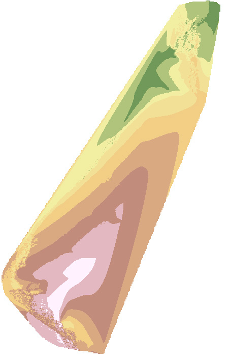
Interpolated bare earth (ground only) returns from airborne lidar collected over Grand County, Colorado

Exercise overview

• Part One - Getting set up: create a new directory, copy files from bvogt's OutBox
• Part Two - The data: spatial data in text (.txt) file format
• Part Three - Adding and viewing data: Converting text files to Shapefiles
• Part Four - Interpolating: Let the fun begin
• Part Five - To post to your web page

Part One - Getting set up

1. Make a new folder in your ges2050/web folder called ‘lidar’.
2. Paste into this new folder two folders from bvogt’s OutBox that are stored here: OutBox\lidar_point_data\  The folders are called airborne and terrestrial.  
   The airborne folder contains a text file of 2004 lidar flown over Cheesman Lake (sw of Denver). The folder also contains two metadata files.
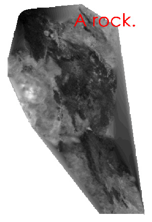
   The terrestrial folder contains two text files of terrestrial lidar: Both are sandstone rock art panels in southeast Colorado (Two Buttes area and Vogel Canyon area). Both panels were scanned by East Carolina University geographer Thad Wasklewicz in 2005 using a Leica-Geosystems terrestrial laser scanner (TLS).

Part Two - The data

• Lidar (Light Detection and Ranging) is a remote sensing technology that collects 3D point clouds from a target (a surface). To collect airborne lidar data, an airplane-mounted instrument uses a laser to transmit and receive pulses of light. From the time delay between light pulse transmission and reception, elevation values from surfaces (buildings, trees, roads, bare earth, water surfaces, glaciers, you, etc.) are calculated. Terrestrial (tripod-mounted) lidar works the same way - only the instrument is generally looking to the side (to see a building) or up (to see the bottom of a highway overpass).
• Text files (.txt) are a fairly common format for importing multispectral lidar point data into GIS and remote sensing software environments. The files contain fields (columns) of x, y, and z data, separated by spaces or commas (in this exercise, the fields in the text files are comma delimited). With terrestrial lidar point data, z values typically represent the distance from the scanner head, whereas with airborne lidar point data, z values generally represent a ground or near ground elevation.
• For this exercise, the airborne lidar dataset (lidar_co.txt) contains x, y, and z data of an urban area near Denver, CO. The terrestrial lidar datasets are a bit different: Both files (twobuttes.txt and vogel.txt) contain x, y, z, i (laser intensity), r (red), g (green), and b (blue) data of rock art (e.g., petroglyph) panels in southeast CO. Attributes i, r, g, and b can be mapped to the location data (x, y, z) in ArcMap and ArcScene to create near photo-quality scenes of the targets.

Part Three - Adding and viewing data: Converting text files to Shapefiles

1. Start with the airborne data. First, open Notepad. From Notepad, open the lidar_co.txt text file.  See for yourself… just x, y, z values with column headers x, y, z. Close Notepad (save nothing). As you can imagine, these files are easy to create from other types of spatial data, including GPS data.
2. Open ArcMap. Turn on Spatial Analyst Extension (Customize > Extensions (check Spatial Analyst), close).
3. Turn on Spatial Analyst Toolbar (Customize > Toolbars > Spatial Analyst). The Spatial Analyst toolbar should appear in your project window.
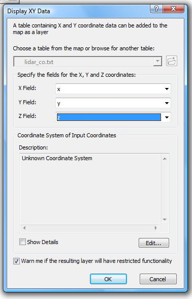
4. In ArcMap, add the text file (Add data > lidar_co.txt). Note that the new file in the Table of Contents is NOT a Shapefile; it is a simple table.
5. Next, right click on the lidar_co.txt file in the Table of Contents and select ‘Display X,Y Data’.  Leave the defaults, but point the ‘Z Field’ to z (use the pull down menu). Click OK.
6. Now you have a new file called ‘lidar_co.txt Events’. Next we'll convert this file to a new Shapefile (you have done this in earlier labs).
7. Right click on the 'lidar_co.txt Events' file in the Table of Contents. Go to Data > Export Data (save to a Shapefile format). Save this new Shapefile to your Z: drive's 'lidar' folder.
8. IMPORTANT: Change the name in the table of contents to “Airborne Lidar Data." Remove the other two files from the Table of Contents (lidar_co.txt Events and lidar_co.txt).
9. Your project should look like this (though colors may vary). SAVE your project (to your z: drive).
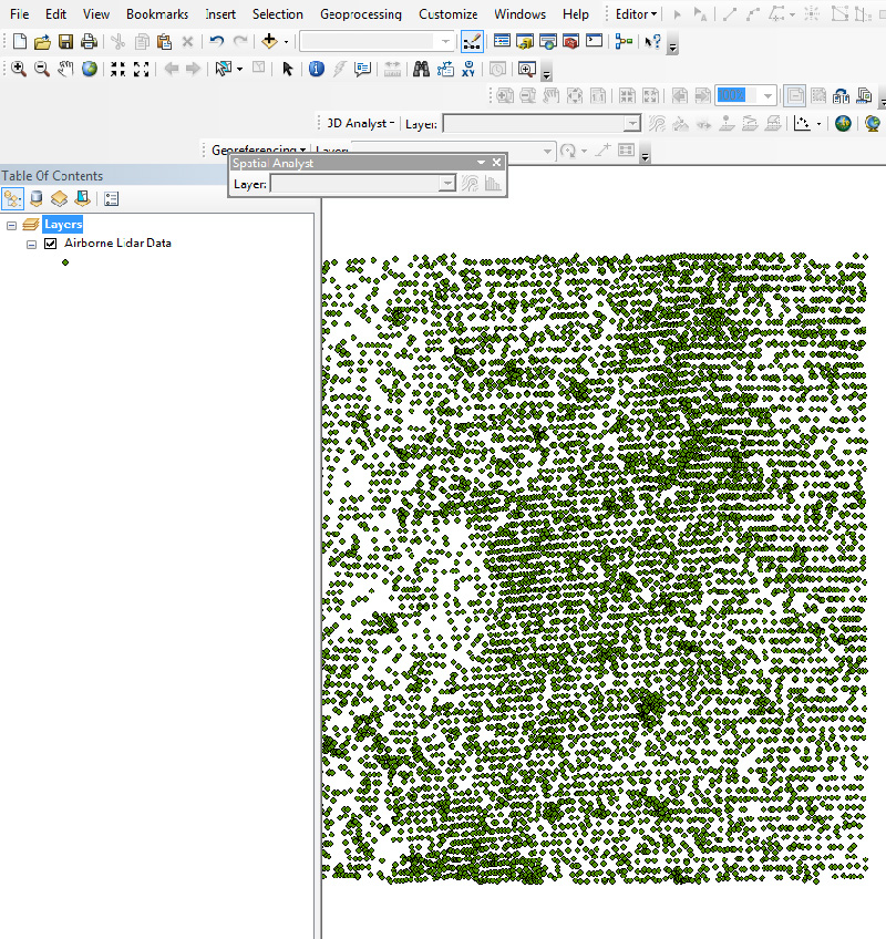
10. Moving on to terrestrial lidar datasets: Repeat the above steps 4 - 9 (add data, display data and point to 'Z' field, convert to Shapefile) for the two terrestrial lidar datasets. As Shapefiles, rename the terrestrial lidar map layers something like "Vogel Terrestrial Lidar Data" and "Two Buttes Terrestrial Lidar Data." Your project, with THREE Shapefiles in the Table of Contents, should look like this.
11. To view the individual files in ArcMap, right - click on the layer in the Table of Contents and select 'Zoom to Layer'.

Part Four - Interpolating... let the fun begin
NOTE: NO SPACES IN FILE / FOLDER NAMES (spaces / funny characters in a path will cause '999999' errors when creating rasters in ArcMap).

1. First: Airborne data: Open ArcToolBox. Go: Spatial Analyst Tools > Interpolation.  Select (open) Natural Neighbor.
2. Set the ‘Input point features’ to your Airborne Lidar Data file (a Shapefile).  Set the Z value field to X. Leave all other setting as default.
3. Repeat the interpolation process two more times: The first time set the Z value field to Y and the second time set the Z value field to Z.  You should now have THREE new raster images (the products of interpolating your airborne lidar data)
4. Notice that one image is a set of vertical lines and one is a set of horizontal lines. Also, one should look like a true surface, irregular and bumpy! You are on the right track now!
5. Remove the two rasters from your project that contain the horizontal and vertical lines (save the one with the bumps)!
6. From the Table of Contents window, rename the new raster file something like 'Airborne Lidar DEM'
7. Next you'll interpolate the two terrestrial datasets:
8. Second: Terrestrial data (Two Buttes): From ArcToolBox. Go: Spatial Analyst Tools > Interpolation.  Again, pick Natural Neighbor.
9. Set the ‘Input point features’ to your 'Two Buttes Terrestrial Lidar Data' Shapefile.  Set the Z value field to Z.
10. Rename the new raster file something like 'Two Buttes Lidar DEM'
11. Third: Terrestrial data (Vogel): From ArcToolBox. Go: Spatial Analyst Tools > Interpolation.  Again, pick Natural Neighbor.
12. Set the ‘Input point features’ to your 'Vogel Terrestrial Lidar Data' Shapefile.  Set the Z value field to Z.
13. Rename the new raster file something like 'Vogel Lidar DEM'
14. Now you should have SIX files in your Table of Contents: 3 point Shapefiles and 3 raster DEM-like (interpolated) images of those points.
15. MAKE SURE THEY ARE ALL NAMED ACCORDINGLY IN THE TABLE OF CONTENTS!
16. To view the individual files in ArcMap, right - click on the layer in the Table of Contents and select 'Zoom to Layer'.

Part Five - To include on your web page

1) MEASUREMENT: In ArcMap, open the Vogel Shapefile's Attribute Table (from Table of Contents, right-click on the Shapefile and select 'Open Attribute Table'). Knowing that the 'z' value is the distance from the scanner head (you read about this earlier in Part Two), measure the difference in meters (units are in meters) from the closest z to the farthest z (round your answer to the nearest 1/100th of a meter (cm). To do this, you need to sort the z values in the Attribute Table twice -- 'Sort Ascending' and 'Sort Descending'.

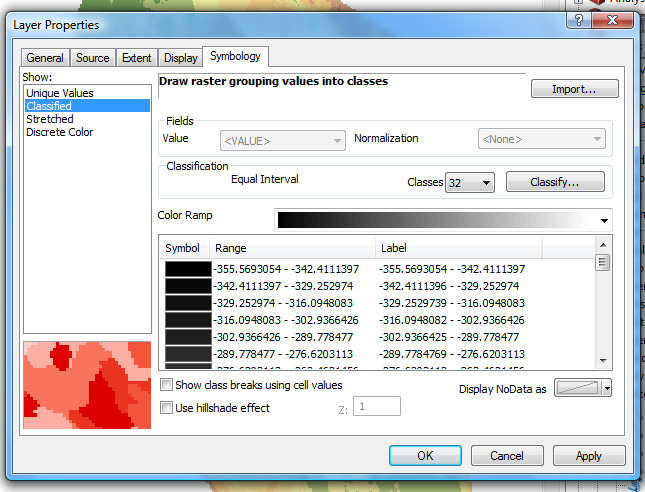
2) IMAGE ONE (with caption): In ArcMap, interpolate using Natural Neighbor the Vogel Shapefile (again) only this time SET THE Z VALUE FIELD TO i (laser intensity). Right-click on the new file, go to the Layer Properties Symbology tab and use these settings. Your new image should resemble (roughly) albedo (reflectivity). Save this image and post it to your web page.

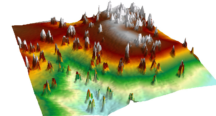
3) IMAGE TWO (with caption): In ArcScene, drape the interpolated airborne lidar image (which is actually a DEM) over itself (get surface heights from the interpolated DEM). You learned this method in Lab Five. Pick any view of this file and post it to your web page.

4) QUESTION ONE: Imagine that your goal is to create a DEM of the UCCS campus using GPS data. Hypothetically, if you had 20 GPS waypoints (x, y, z) collected from across campus, Notepad, and ArcMap, briefly go through ALL OF THE KEY STEPS you would need to follow to make a DEM (raster) of the UCCS campus from start to finish.

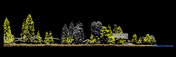
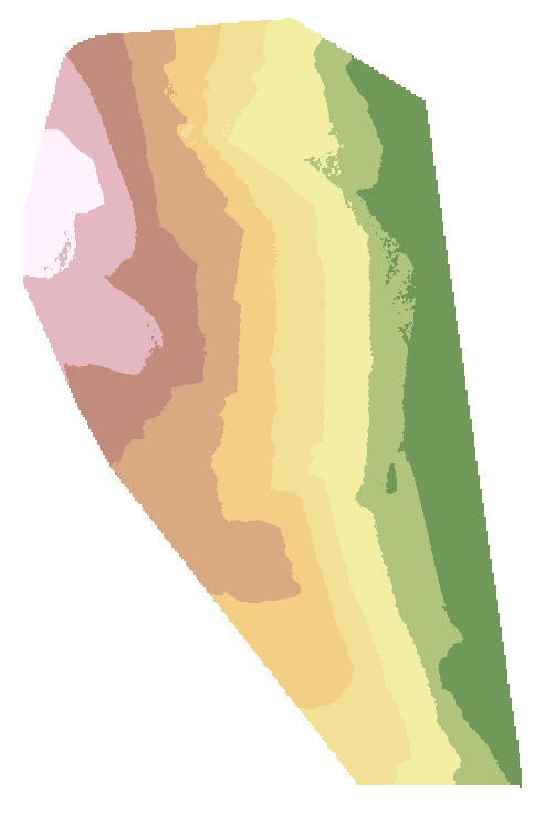
Several classes of airborne lidar data along a cabin-lined stream, Grand Lake, Colorado