Rates of Change and the Tangent Line

Tangent Lines

Let's take a look at the process that we're doing in Example 2. If we graph $f(t)$ and plot the two points we're using for our average velocity calculation, we can connect those points with a line that touches $f(t)$ in two places. Then, we can view our average velocity as the slope of that line. In the demonstration below, drag the orange point closer to the point at $(0.8, 63.36)$. Observe what happens to the average velocity as these points get closer together. Also observe what happens to the line connecting the points.

We have a special name for that line; it's called the secant line.

A secant line might look something like this.

Note: The following content is adapted from Paul's Online Math Notes, with permission, and is not shared under the Creative Commons license.

Before moving on let's do a quick review of just what we did in the above example using this new point of view where we think about lines instead of just velocities. We started with the point $P=(a,f(a))$ as a point we know is on the tangent line. Next, we took a second point that is on the graph of the function and called it $Q = (b,f(b))$. With these two points, we computed the slope of the line connecting $P$ and $Q$ using the formula \[m_{PQ} = \dfrac{f(x)-f(a)}{x-a}.\]

We then took values of $t$ that got closer and closer to $t = a$ (making sure to look at $t$-values on both sides of $t = a$), and we used this list of values to estimate the an instantaneous slope, $m$.

We will call the line at $t = a$ with instantaneous slope $m$ the tangent line. The tangent line then had equation $y = m(x-a) + f(a)$.

Take a look at the graph below.

In this graph the line is a tangent line at the first indicated point because it just touches the graph at that point. Likewise, at the second point shown, the line goes through the same point as the graph of $f(x)$, but in a different direction than $f(x)$, so it's not a tangent line to the graph at that point.

We can think about the tangent line as being formed by creating a secant line through two points, and then moving one of those points closer and closer to the other. In the demonstration below, you can adjust the h slider to move the red point closer to the blue point. As you do this, the secant line through the two points looks more and more like the tangent line through the blue point.

Now that we have loosely defined the tangent line, let's move on to the tangent line problem with an example.

Find the equation of the tangent line to the graph of $f(x)=15-2x^2$ at $x = 1$.

Click for solution

To find an equation of a line we need either two points on the line or a single point on the line and the slope of the line. Since we know that we are after a tangent line we can use $f(x)$ to find the point where the line must touch the graph of the function. Specifically, the tangent line and the graph of the function must touch at $x = 1$, so we plug $x = 1$ into the formula $f(x) = 15-2x^2$ to get the $y$-value of $f(1) = 15-2(1)^2 = 13$. So the point $(1,13)$ must be on the tangent line.

Now we reach the tangent line problem. In order to find the tangent line we need either a second point or the slope of the tangent line. Since we want the tangent line to go in the same direction as $f(x)$ at $(1,13)$, we will concentrate on attempting to determine the slope of the tangent line.

At this point in time, all we can do with certainty is estimate the slope of the tangent line, but if we can find a pattern in our estimates, we may be able to find the actual slope of the tangent line, not just an estimate. We'll do this by starting with the point that we already have on the line, let's call it $P = (1,13)$.

To estimate slope, we need two points, so we will then pick another point that lies on the graph of the function; let's call that point $Q = (x,f(x))$. For example, if $x = 2$, then the second point will be $Q = (2,7)$ since $f(2) = 15-2(2)^2 = 7$.

Below is a graph of the function, the tangent line, and the secant line that connects $P$ and $Q$.

We can see from this graph that the secant and tangent lines are somewhat similar and so the slope of the secant line should be somewhat close to the actual slope of the tangent line. So, as an estimate of the slope of the tangent line we can use the slope of the secant line. Let's call the slope of the secant line $m_{PQ}$, which is \[m_{PQ} = \dfrac{f(2)-f(1)}{2-1} = \dfrac{7-13}{2-1} = -6.\]

Now, this is one estimate for the slope of the tangent line, but we can do better. To improve the estimate, we can take $x$ closer to $x = 1$ and redo the above work to get a new estimate on the slope. We could then repeat the process with a yet closer $x$ value to get an even better estimate.

In other words, as we take $Q$ closer and closer to $P$, the slope of the secant line connecting $Q$ and $P$ should be getting closer and closer to the slope of the tangent line. Below you can see many different secant lines through $(1,13)$ whose slopes are getting closer and closer to the tangent line.

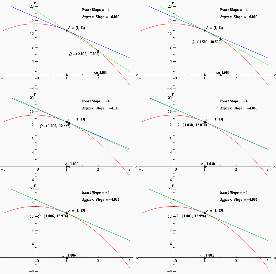
As we move $Q$ closer and closer to $P$, the secant lines do start to look more and more like the tangent line and so the approximate slopes (i.e. the slopes of the secant lines) are getting closer and closer to the exact slope.

In this figure we only looked at points $Q$ that were to the right of $P$, but we could have just as easily used points that were to the left of $P$ and we would have received the same results. In fact, we should always take a look at points that are on both sides of $P$, since these could give us different results (and we will eventually see examples of this in future sections). Remember to always look at what is happening on both sides of the point in question when doing this kind of process.

Now, let's find the approximate slopes showed in the graph above, and hence an estimation of the slope of the tangent line. In order to simplify the process a little, let's write down a formula for the slope of the line between $P$ and $Q$, $m_{PQ}$, that will work for any $x$ that we choose to work with. Since the slope is between $P = (1,13)$ and $Q = (x,f(x))$, the formula for $m_{PQ}$ is \[m_{PQ} = \dfrac{f(x)-f(1)}{x-1} = \dfrac{15-2x^2-13}{x-1} = \dfrac{2-2x^2}{x-1}.\]

Now let's make a table of the slope $m_{PQ}$ at specific $x$-values getting closer and closer to $x = 1$.

$$\begin{array}{l|l} x & m_{PQ} \\ \hline 2 & -6 \\ 1.5 & -5 \\ 1.1 & -4.2 \\ 1.01 & -4.02\\ 1.001 & -4.002 \\ 1.0001 & -4.0002 \\ \end{array}\hspace{2em} \begin{array}{l|l} x & m_{PQ} \\ \hline 0 & -2 \\ 0.5 & -3 \\ 0.9 & -3.8 \\ 0.99 & -3.98 \\ 0.999 & -3.998 \\ 0.9999 & -3.9998 \\ \end{array}$$

So, if we take $x$-values to the right of $x = 1$ and take them closer and closer to $x = 1$, it appears that the slope of the secant lines is approaching $-4$. Likewise, if we take $x$-values to the left of $x = 1$ and take them closer and closer to $x = 1$, it appears the slope of the secant lines is again approaching $-4$.

Based on this evidence, the slopes of the secant lines are approaching $-4$ as the $x$-values of $Q$ approach $x = 1$ from both the left and the right sides, so we will estimate that the slope of the tangent line is also $-4$. We will eventually be able to prove that this is the slope of the tangent line and not just guess from a pattern on a table.

As a reminder, the equation of the line that goes through $(a,f(a))$ with slope $m$ is given by $y = m(x-a) + f(a)$.

Therefore, since the tangent line goes through $(1,13)$ and we just estimated its slope as $m = -4$, the equation of the tangent line to the graph of $f(x) = 15-2x^2$ at $x = 1$ is \[y = -4(x-1)+13.\]

Use the below practice to try this a few times before moving on to the next topic of this section.

For the function $f(x) = 3(x+2)^2$ and the point $P$ given by $x=-3$ answer each of the following questions.

1. For the points $Q$ given by the following values of $x$ compute (accurate to at least 8 decimal places) the slope, $m_{PQ}$, of the secant line through points $P$ and $Q$.
1. -3.5
2. -3.1
3. -3.01
4. -3.001
5. -3.0001
1. -2.5
2. -2.9
3. -2.99
4. -2.999
5. -2.999
2. Use the information from (a) to estimate the slope of the tangent line to $f(x)$ at $x=-3$ and write down the equation of the tangent line.

Click for solution

a. The first thing that we need to do is set up the formula for the slope of the secant lines. As discussed in this section this is given by, $$m_{PQ}=\frac{f(x)-f(-3)}{x-(-3)} = \frac{3(x+2)^2-3}{x+3}.$$

Now, all we need to do is construct a table of the value of $m_{PQ}$ for the given values of $x$. All of the values in the table below are accurate to 8 decimal places, but in this case the values terminated prior to 8 decimal places and so the “trailing” zeros are not shown.

$$\begin{array}{c|c} x & m_{PQ}\\ \hline -3.5 & -7.5 \\ -3.1 & -6.3\\ -3.01 & -6.03\\ -3.001 & -6.003\\ -3.0001 & -6.0003\\ \end{array} ~~~~~~~~~~~~ \begin{array}{c|c} x& m_{PQ}\\ \hline -2.5 & -4.5\\ -2.9 & -5.7\\ -2.99 & -5.97\\ -2.999 & -5.997\\ -2.9999 & -5.9997\\ \end{array}$$

---

b. From the table of values above we can see that the slope of the secant lines appears to be moving towards a value of -6 from both sides of $x=-3$ and so we can estimate that the slope of the tangent line is: $m = -6$.

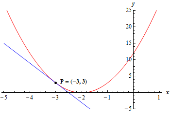
The equation of the tangent line is then $$y = f(-3) + m(x-(-3)) = 3 - 6(x+3) ~~~~~\Rightarrow ~~~~~ y = -6x - 15.$$

Here is a graph of the function and the tangent line.

Rates of Change

The next problem that we need to look at is the rate of change problem. As mentioned earlier, this will turn out to be one of the most important concepts that we will look at throughout this course, and it is very closely related to the tangent line problem.

Let's consider a function $f(x)$ that represents some quantity that varies as $x$ varies. For instance, maybe $f(x)$ represents the amount of water in a holding tank after $x$ minutes. Or maybe $f(x)$ is the distance traveled by a car after $x$ hours. In both of these example we used $x$ to represent time. Of course $x$ doesn't have to represent time, but it makes for examples that are easy to visualize. We can also use input variables other than $x$.

To compute the average rate of change of $f(x)$ at $x = a$, all we need to do is to choose another point, say $x$, and then the average rate of change will be \[\text{average rate of change} = \dfrac{\text{change in } f(x)}{\text{change in }x} = \dfrac{f(x)-f(a)}{x-a}.\]

This may remind you of the slope calculations we did earlier in this section (remember that slope simply measures change in output divided by change in input).

To estimate the instantaneous rate of change at $x = a$, all we need to do is to choose values of $x$ getting closer and closer to $x = a$ (don't forget to choose them on both sides of $x = a$) and compute values of $\dfrac{f(x)-f(a)}{x-a}$. We can then estimate the instantaneous rate of change from these values.

Let's take a look at an example.

We can also interpret what these rates of change mean. At $t = 4$, the rate of change is zero, and so at this point in time the volume is not changing at all. That doesn't mean that it will not change in the future. It just means that exactly at $t = 4$ the volume isn't changing. Likewise, at $t = 3$ the volume is decreasing since the rate of change at that point is negative. We can also say that, regardless of the increasing/decreasing aspects of the rate of change, the volume of the balloon is changing faster at $t = 5$ than it is at $t = 3$ since 15 is larger than -9.

We will be talking a lot more about rates of change when we get into the next chapter.

The Velocity Problem

One specific example of the rate of change problem that is often studied in calculus books is the velocity problem. In the velocity problem we are given a position function of an object, $f(t)$, that gives the position of an object at time $t$ along an axis. For instance, think about a car driving down a highway and $f(t)$ measures how far it has traveled on that highway. Then to compute the instantaneous velocity of the object we just need to recall that the velocity is nothing more than the rate at which the position is changing.

In other words, to estimate the instantaneous velocity of the object at time $t = a$ we would first compute the average velocity, \[\text{average velocity} = \dfrac{\text{change in position}}{\text{time traveled}} = \dfrac{f(t)-f(a)}{t-a}\] and then take values of $t$ closer and closer to $t = a$ and use these values to estimate the instantaneous velocity.

Alternate Notation

There is one last bit of notation that we will cover in this section before we move on. The main point of this section was to introduce us to a couple of key concepts and ideas that we will see throughout the first portion of this course as well as get us started down the path towards limits and eventually derivatives.

Instead of having two points with totally different inputs, $(a,f(a))$ and $(x,f(x))$, we are going to focus on the point $(a,f(a))$ and a second point defined relative to it. Suppose we want to move on the $x$-axis a distance of $h$ from $x = a$. Then our new $x$ value is $x = a+h$. This is shown below in a sketch.

...now we'll think about a point of interest at $a$ and another point that is $h$ units away.

For instance, if $a = 5$ and $h = 0.1$, then $a + h = 5 + 0.1 = 5.1$, an $x$-value a little bit to the right of $x = 5$. Likewise, if $h = -0.01$, then $a+h = 5-0.01 = 4.99$ for these example numbers, an $x$-value a little bit to the left of $x = 5$. Moreover, as $h$ gets closer and closer to $0$, $a+h$ is getting closer and closer to $a$.

As we noted earlier in this section, it is important to take values of $x$ that are on both sides of $x = a$. We can do that with this new way of choosing $x = a+h$, since choosing $h \gt0$ will cause $x = a+h$ to be an $x$-value right of $x=a$, while choosing $h \lt 0$ will cause $x = a+h$ to be an $x$-value left of $x=a$.

Now, with this new way of obtaining a second $x$-value, namely $\textcolor{blue}{x = a+h}$, the difference quotient becomes \[\dfrac{f(\textcolor{blue}{x})-f(a)}{\textcolor{blue}{x}-a} = \dfrac{f(\textcolor{blue}{a+h})-f(a)}{\textcolor{blue}{a+h}-a} = \dfrac{f(a+h)-f(a)}h.\]

This is for a specific value of $x$, i.e., $x = a$ (for example, $x = 5$ or $x = -2.1$). If we want to look at a difference quotient centered at the general value of $x$, we simply replace $a$ with $x$ to get \[\dfrac{f(x+h)-f(x)}h.\]

Below is an interactive example to illustrate. As you move the h slider closer to 0, point B moves closer to point A.

Let's see how we can apply this definition to some of our previous examples.

We won't dictate which method you should use to make these calculations, for now. Experiment with each version to get a better understanding of how they're similar and how they're different.

Practice Problems

1. For the function $g(x) = \sqrt{4x+8}$ and the point $P$ given by $x=2$, answer each of the following questions.
   1. For the points $Q$ given by the following values of $x$, compute (accurate to at least 8 decimal places) the slope, $m_{PQ}$, of the secant line through points $P$ and $Q$.
   1. 2.5
   2. 2.1
   3. 2.01
   4. 2.001
   5. 2.0001
   6. 1.5
   7. 1.9
   8. 1.99
   9. 1.999
   10. 1.999
   2. Use the information from (a) to estimate the slope of the tangent line to $g(x)$ at $x=2$ and write down the equation of the tangent line.
   Click for solution
   

   1. The first thing that we need to do is set up the formula for the slope of the secant lines. As discussed in this section this is given by,

      $$m_{PQ} = \frac{g(x)-g(2)}{x-2} = \frac{\sqrt{4x+8}-4}{x-2}.$$

      Now, all we need to do is construct a table of the value of $m_{PQ}$ for the given values of $x$. All of the values in the table below are accurate to 8 decimal places.

      $$\begin{array}{c|c} x & m_{PQ}\\ \hline 2.5 & 0.48528137\\ 2.1 & 0.49691346\\ 2.01 & 0.49968789\\ 2.001 & 0.49996875\\ 2.0001 & 0.49999688\\ \end{array} ~~~~~~~~ \begin{array}{c|c} x & m_{PQ}\\ \hline 1.5 & 0.51668523\\ 1.9& 0.50316468\\ 1.99 & 0.50031289\\ 1.999 & 0.50003125\\ 1.9999 & 0.50000313 \\ \end{array} $$
      

      ---

      
      
   2. From the table of values above we can see that the slope of the secant lines appears to be moving towards a value of 0.5 from both sides of $x=2$ and so we can estimate that the slope of the tangent line is $m = 0.5 = \frac12$.

      The equation of the tangent line is then, $$y = g(2)+m(x-2) = 4+\frac12(x-2) ~~~\Rightarrow ~~~ y = \frac12x + 3.$$

   
   
2. For the function $W(x)=\ln(1+x^4)$ and the point $P$ given by $x=1$, answer each of the following questions.
   1. For the points $Q$ given by the following values of $x$, compute (accurate to at least 8 decimal places) the slope, $m_{PQ}$, of the secant line through points $P$ and $Q$.
      1. 1.5
      2. 1.1
      3. 1.01
      4. 1.001
      5. 1.0001

      6. 0.5
      7. 0.9
      8. 0.99
      9. 0.999
      10. 0.999
   2. Use the information from (a) to estimate the slope of the tangent line to $g(x)$ at $x=2$ and write down the equation of the tangent line.
   Click for solution
   

   1. The first thing that we need to do is set up the formula for the slope of the secant lines. As discussed in this section this is given by,

      $$m_{PQ} = \frac{W(x)-W(1)}{x-1} = \frac{\ln(1+x^4)-\ln(2)}{x-1}.$$

      Now, all we need to do is construct a table of the value of $m_{PQ}$ for the given values of $x$. All of the values in the table below are accurate to 8 decimal places.

      $$\begin{array}{c|c} x & m_{PQ}\\ \hline 1.5 & 2.21795015\\ 1.1 & 2.08679449\\ 1.01 & 2.00986668\\ 1.001 & 2.00099867 \\ 1.0001 & 2.00009999\\ \end{array} ~~~~~~~~ \begin{array}{c|c} x & m_{PQ}\\ \hline 0.5 & 1.26504512\\ 0.9& 1.88681740\\ 0.99 & 1.98986668\\ 0.999 & 1.99899867\\ 0.9999 & 1.99989999 \\ \end{array} $$
      

      ---

      
      
   2. From the table of values above we can see that the slope of the secant lines appears to be moving towards a value of 2 from both sides of $x=1$ and so we can estimate that the slope of the tangent line is $m = 2$.

      The equation of the tangent line is then, $$y = W(1)+m(x-1) = \ln(2)+2(x-1).$$



3. The position of an object is given by $s(t) = \cos^2\left(\frac{3t-6}{2}\right)$. Answer each of the following questions.
   1. Compute (accurate to at least 8 decimal places) the average velocity of the object between $t=2$ and the following values of $t$. Make sure your calculator is set to radians for the computations.
      1. 2.5
      2. 2.1
      3. 2.01
      4. 2.001
      5. 2.0001

      6. 1.5
      7. 1.9
      8. 1.99
      9. 1.999
      10. 1.999
   2. Use the information from (a) to estimate the instantaneous velocity of the object at $t=2$ and determine if the object is moving to the right (i.e. the instantaneous velocity is positive), moving to the left (i.e. the instantaneous velocity is negative), or not moving (i.e. the instantaneous velocity is zero).
   Click for solution
   
   1. The first thing that we need to do is set up the formula for the average velocity. As discussed in this section this is given by,
      $$A.V.=\frac{s(t)-s(2)}{t-2} = \frac{\cos^2\left(\frac{3t-6}{2}\right)-1}{t-2}.$$ Now, all we need to do is construct a table of the value of $A.V.$ for the given values of $t$. All of the values in the table below are accurate to 8 decimal places.
      $$\begin{array}{c|c} t & A.V.\\ \hline 2.5 & -0.92926280\\ 2.1 & -0.22331755\\ 2.01 & -0.02249831\\ 2.001 & -0.00225000 \\ 2.0001 & -0.00022500\\ \end{array} ~~~~~~~~ \begin{array}{c|c} t & A.V.\\ \hline 1.5 & 0.92926280\\ 1.9& 0.22331755\\ 1.99 & 0.02249831\\ 1.999 & 0.00225000\\ 1.9999 & 0.00022500 \\ \end{array} $$
      

      ---

      
      
   2. From the table of values above we can see that the average velocity of the object is moving towards a value of 0 from both sides of $t=2$ and so we can estimate that the instantaneous velocity is 0 and so the object will not be moving at $t=2$.

Assignment Problems

1. For the function $f(x)=x^3-3x^2$ and the point $P$ given by $x=3$, answer each of the following questions.
   1. For the points $Q$ given by the following values of $x$, compute (accurate to at least 8 decimal places) the slope, $m_{PQ}$, of the secant line through points $P$ and $Q$.
      1. 3.5
      2. 3.1
      3. 3.01
      4. 3.001
      5. 3.0001

      6. 2.5
      7. 2.9
      8. 2.99
      9. 2.999
      10. 2.999
   2. Use the information from (a) to estimate the slope of the tangent line to $f(x)$ at $x=3$ and write down the equation of the tangent line.


2. For the function $g(x) = \frac{x}{x^2+4}$ and the point $P$ given by $x=0$, answer each of the following questions.
   1. For the points $Q$ given by the following values of $x$, compute (accurate to at least 8 decimal places) the slope, $m_{PQ}$, of the secant line through points $P$ and $Q$.
      1. 1
      2. 0.5
      3. 0.1
      4. 0.01
      5. 0.001

      6. -1
      7. -0.5
      8. -0.1
      9. -0.01
      10. -0.001
   2. Use the information from (a) to estimate the slope of the tangent line to $g(x)$ at $x=0$ and write down the equation of the tangent line.


3. For the function $h(x) = 2-(x+2)^2$ and the point $P$ given by $x=-2$, answer each of the following questions.
   1. For the points $Q$ given by the following values of $x$, compute (accurate to at least 8 decimal places) the slope, $m_{PQ}$, of the secant line through points $P$ and $Q$.
      1. -2.5
      2. -2.1
      3. -2.01
      4. -2.001
      5. -2.0001

      6. -1.5
      7. -1.9
      8. -1.99
      9. -1.999
      10. -1.9999
   2. Use the information from (a) to estimate the slope of the tangent line to $h(x)$ at $x=-2$ and write down the equation of the tangent line.


4. For the function $P(x) = e^{2-8x^2}$ and the point $P$ given by $x=0.5$, answer each of the following questions.
   1. For the points $Q$ given by the following values of $x$, compute (accurate to at least 8 decimal places) the slope, $m_{PQ}$, of the secant line through points $P$ and $Q$.
      1. 1
      2. 0.51
      3. 0.501
      4. 0.5001
      5. 0.50001

      6. 0
      7. 0.49
      8. 0.499
      9. 0.4999
      10. 0.49999
   2. Use the information from (a) to estimate the slope of the tangent line to $h(x)$ at $x=0.5$ and write down the equation of the tangent line.


5. The amount of grain in a bin is given by $V(t) = \frac{11t+4}{t+4}$. Answer each of the following questions.
   1. Compute (accurate to at least 8 decimal places) the average rate of change of the amount of grain in the bin between $t=6$ and the following values of $t$.
      1. 6.5
      2. 6.1
      3. 6.01
      4. 6.001
      5. 6.0001

      6. 5.5
      7. 5.9
      8. 5.99
      9. 5.999
      10. 5.9999
   2. Use the information from (a) to estimate the instantaneous rate of change of the volume of grain in the bin at $t=6$.


6. The population (in thousands) of insects is given by $P(t) = 2-\frac{1}{\pi}\cos(3\pi t)\sin\left(\frac{\pi t}{2}\right)$. Answer each of the following questions.
   1. Compute (accurate to at least 8 decimal places) the average rate of change of insects between $t=4$ and the following values of $t$. Make sure your calculator is set to radians for the computations.
      1. 4.5
      2. 4.1
      3. 4.01
      4. 4.001
      5. 4.0001

      6. 3.5
      7. 3.9
      8. 3.99
      9. 3.999
      10. 3.9999
   2. Use the information from (a) to estimate the instantaneous rate of change of the population of insects at $t=4$.


7. The amount of water in a holding tank is given by $V(t) = 8t^4-t^2+7$. Answer each of the following questions.
   1. Compute (accurate to at least 8 decimal places) the average rate of change of the amount of water in the tank between $t=0.25$ and the following values of $t$.
      1. 1
      2. 0.5
      3. 0.251
      4. 0.2501
      5. 0.25001

      6. 0
      7. 0.1
      8. 2.49
      9. 2.499
      10. 2.4999
   2. Use the information from (a) to estimate the instantaneous rate of change of the volume of water in the tank at $t=0.25$.


8. The position of an object is given by $s(t) = t^2 + \frac{72}{t+1}$. Answer each of the following questions.
   1. Compute (accurate to at least 8 decimal places) the average velocity of the object between $t=5$ and the following values of $t$.
      1. 5.5
      2. 5.1
      3. 5.01
      4. 5.001
      5. 5.0001

      6. 4.5
      7. 4.9
      8. 4.99
      9. 4.999
      10. 4.9999
   2. Use the information from (a) to estimate the instantaneous velocity of the object at $t=5$ and determine if the object is moving to the right (i.e. the instantaneous velocity is positive), moving to the left (i.e. the instantaneous velocity is negative), or not moving (i.e. the instantaneous velocity is zero).


9. The position of an object is given by $s(t) = 2\cos(4t-8)-7\sin(t-2)$. Note that a negative position here simply means that the position is to the left of the “zero position” and is perfectly acceptable Answer each of the following questions.
   1. Compute (accurate to at least 8 decimal places) the average velocity of the object between $t=2$ and the following values of $t$. Make sure your calculator is set to radians for the computations.
      1. 2.5
      2. 2.1
      3. 2.01
      4. 2.001
      5. 2.0001

      6. 1.5
      7. 1.9
      8. 1.99
      9. 1.999
      10. 1.9999
   2. Use the information from (a) to estimate the instantaneous velocity of the object at $t=2$ and determine if the object is moving to the right (i.e. the instantaneous velocity is positive), moving to the left (i.e. the instantaneous velocity is negative), or not moving (i.e. the instantaneous velocity is zero).
   
   
10. The position of an object is given by $s(t) = t^2 + \frac{72}{t+1}$. Answer each of the following questions.
1. Determine the time(s) in which the position of the object is at $s=-5$.
2. Estimate the instantaneous velocity of the object at each of the time(s) found in part (a) using the method discussed in this section.