The Shape of a Graph, Part 2
Click here for a printable version of this page.Concavity and Inflection Points
In the previous section, we used the first derivative to find information about the graph of a function. In this section, we will use the second derivative to gain more refined information about the shape of the graph.
The main concept that we'll be discussing in this section is concavity. We will give the formal definition soon, but first let's take a look at concavity on a few graphs.

We describe a graph as concave up if it "opens" upwards, and concave down if it "opens" downwards. Notice from these four examples that concavity has nothing to do with whether the graph is increasing or decreasing. That is, a graph may be concave up and either increasing or decreasing. Similarly, a graph may be concave down and either increasing or decreasing.
While "opens" upwards or downwards is a way to describe concavity that might evoke the right image, it is not very useful as a definition. Here is the formal mathematical definition of the two types of concavity.
Definition of Concavity
Given a function $f(x),$ we say that- $f(x)$ is concave up on an interval $I$ if the graph of $y=f(x)$ lies above all of its tangent lines at every $x\in I.$
- $f(x)$ is concave down on an interval $I$ if the graph of $y=f(x)$ lies below all of its tangent lines at every $x\in I.$
Here are the graphs from the image above, with some of the tangent lines sketched on them.

We can see that, in the upper two graphs, all of the tangent line segments are below the graphs and the graphs are concave up, while in the lower two graphs, which are concave down, the tangent line segments lie above the graphs.
Again we notice that concavity and the increasing/decreasing behavior of the functions are completely independent. This is important to remember because students often mix the two and try to use information about one to find information about the other, which leads to incorrect information about the graph.
Just as a point where a function changes from increasing to decreasing (or vice-versa) is an important point on a graph, so is a point where the concavity changes. Here is the definition of such a point.
Definition of Inflection Point
A point $(c, f(c))$ is called an inflection point of $f(x)$ if the function is continuous at the point and the concavity of the graph changes at that point.Now is the time to bring the second derivative into the picture. After all, the goal of this section is to understand the relationship between the second derivative of a function and the graph of the function. The following fact relates the second derivative of a function to the concavity of the graph.
We are stating the fact as a theorem, but it is really another corollary to the Mean Value Theorem. We will discuss the Mean Value Theorem fully in the next section, and will provide a proof of it there. In the proof of the statement below, all we need is the conclusion of the Mean Value Theorem.
Theorem
Let $f(x)$ be a function whose second derivative exists on some interval $I.$- If $f''(x)\gt 0$ for all $x$ in $I,$ then $f(x)$ is concave up on $I.$
- If $f''(x) \lt 0$ for all $x$ in $I,$ then $f(x)$ is concave down on $I.$
Proof of statement 1
Let $f(x)$ be a function that is twice differentiable on an interval $I,$ and suppose that $f''(x)\gt 0$ for all $x\in I.$ Let $a$ be any number in $I.$ The equation of the tangent line to $f(x)$ at $x=a$ is $$y=f(a) + f'(a)(x-a)$$
To show that $f(x)$ is concave up on $I,$ we need to show that for any $x\in I$ with $x\neq a,$ $$f(x)\gt f(a)+f'(a)(x-a)$$
In other words, we need to show that the tangent line at any point $x=a$ in $I$ is below the graph of $f(x).$ Note that we require $x\neq a$ because at the point where $x=a,$ $f(x)=f(a),$ meaning that at the point of tangency, the tangent line is neither above nor below the graph.
Since $x\neq a,$ the interval $I$ has two pieces, to the left of $a$ and to the right of $a.$ Let's begin by considering the interval to the right of $a;$ that is, we'll assume that $x\gt a.$ Applying the Mean Value Theorem to $f(x)$ on the closed interval $[a,x]$ gives a number $c$ such that $a\lt c\lt x$ and $$f(x)-f(a) = f'(c)(x-a)$$
Rewriting slightly, this becomes
$$f(x) = f(a) + f'(c)(x-a)$$Recall that the hypothesis for this part is that $f''(x)\gt 0$ for all $x\in I.$ This means that the first derivative, $f'(x),$ is increasing on $I$ (because its derivative, $f''(x),$ is positive). We have $a\lt c$ from the statement above, and so by definition of increasing, $$f'(a)\lt f'(c)$$
In addition, because $x\gt a,$ we have $x-a\gt 0.$ Multiplying the inequality above by the positive quantity $x-a$ then yields $$f'(a)(x-a)\lt f'(c)(x-a)$$
Next add $f(a)$ to both sides of this inequality to obtain
$$f(a) + f'(a)(x-a) \lt f(a) + f'(c)(x-a)$$However, in the statement that we obtained from the Mean Value Theorem, we saw that the right side of this inequality is just $f(x).$ So we have
$$f(a) + f'(a)(x-a)\lt f(x)$$But this is exactly what we wanted to show. So, provided that $x\gt a,$ the tangent line at $x=a$ is below the graph of $y=f(x).$
Now let's assume that $x\lt a.$ Applying the Mean Value Theorem to $f(x)$ on the interval $[x,a]$ now gives a number $c$ such that $x\lt c\lt a$ and $$f(a)-f(x) = f'(c)(a-x)$$
Multiplying both sides of this by $-1$ and adding $f(a)$ to both sides yields $$f(x)=f(a)+f'(c)(x-a)$$
Now as we noted above, the fact that $f''(x)\gt 0$ for all $x\in I$ means that the derivative $f'(x)$ is increasing on $I.$ So because $c\lt a,$ we can say that $$f'(c)\lt f'(a)$$
Now since $x\lt a,$ $x-a\lt 0,$ so when we multiply the inequality by $x-a,$ we reverse the inequality symbol, giving $$f'(c)(x-a)\gt f'(a)(x-a)$$
If we now add $f(a)$ to both sides of this inequality, we have $$f(a)+f'(c)(x-a)\gt f(a)+f'(a)(x-a)$$
However, the left side of this inequality is just $f(x),$ so we may conclude that $$f(x)\gt f(a)+f'(a)(x-a)$$
So, provided that $x\lt a,$ the tangent line at $x=a$ is also below the graph of $y=f(x).$
We have shown that for any $a\in I,$ the tangent line at $x=a$ lies below the graph of $y=f(x).$
Therefore, if $f''(x)\gt 0$ for all $x$ in $I,$ $f(x)$ is concave up on $I.$
Proof of statement 2
Let $f(x)$ be a function that is twice differentiable on an interval $I,$ and suppose that $f''(x)\lt 0$ for all $x\in I.$ Let $a$ be any number in $I.$ To show that $f(x)$ is concave down, we need to show that for any $x$ in $I,$ with $x\neq a,$ the tangent line lies above the graph of $f(x).$ That is, we need to show that $$f(x)\lt f(a)+f'(a)(x-a).$$
From here, the proof is nearly identical to the proof of statement 1, except that this time, because $f''(x)\lt 0,$ the derivative $f'(x)$ is decreasing on $I.$ We'll leave it to you to fill in the rest of the proof.
What the theorem tells us is that the inflection points are the points where the second derivative changes sign. We've seen already that a function may change its sign at any point where it is zero or does not exist. So the possible inflection points are those points where the second derivative is zero or does not exist.
Be careful not to assume that every point where the second derivative is zero or doesn't exist is an inflection point, though. These are just the possible inflection points. We need to determine the concavity and see that the concavity is different on either side of the point before we may conclude that the point is, in fact, an inflection point.
Note: The following content is adapted from OpenStax and is licensed under a Creative Commons Attribution-NonCommercial-ShareAlike 4.0 International License.
Access for free at https://openstax.org/books/calculus-volume-1/pages/1-introduction.

Given the function $$f(x) = x^3 - 6x^2 +9x+30,$$ determine all intervals where $f$ is concave up and all intervals where $f$ is concave down. List all inflection points for $f.$
To determine concavity, we need to find the second derivative, $f''(x).$ The first derivative is $$f'(x) = 3x^2-12x+9$$ and the second derivative is $$f''(x) = 6x-12.$$
Since any function changes sign only where it is zero or undefined, this is true of the second derivative. So if the function changes concavity, it occurs either when $f''(x) =0$ or $f''(x)$ is undefined. Since $f''(x)$ is defined for all real numbers (it is a polynomial), we need only find where $f''(x) = 0.$
Solving $6x-12=0,$ we find $x=2$ is the only place where $f$ could change concavity. In other words, it is a possible location of an inflection point. Just as we did with increasing/decreasing behavior, we will use the possible inflection point to divide the number line into intervals, then find the sign of the second derivative at a test point in each interval. Here is the number line showing this:
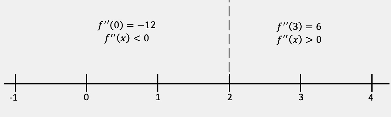
We conclude that $f$ is concave down over the interval $(-\infty,2)$ and concave up over the interval $(2,\infty).$ Since $f$ changes concavity at $x=2,$ the point $(2,f(2)) = (2,32)$ is an inflection point.
Note: The following content is adapted from Paul's Online Math Notes, with permission, and is not shared under the Creative Commons license.
In the next example, we will put together everything we've done in the last section and this section so far to create a pretty accurate graph of a function.
Given the function $$h(x) = 3x^5-5x^3+3,$$ determine all intervals where the function is increasing, the intervals where it is decreasing, and the intervals where it is concave up and the intervals where it is concave down. Identify any relative extrema and inflection points, then sketch the graph.
We will need the first two derivatives, so let's find those first.
\begin{align*} h'(x) &= 15x^4 - 15x^2 = 15x^2(x-1)(x+1)\\ h''(x) &= 60x^3 - 30x = 30x(2x^2-1)\\ \end{align*}First note that the function and its first two derivatives exist for all real $x$ since they are polynomials.
To find the increasing/decreasing behavior and relative extrema of the function, we need the critical numbers. Setting $h'(x)$ equal to zero, we find $x=-1, x=0,$ and $x=1.$ Here is the number line for the first derivative:

So the intervals of increase and intervals of decrease are
$$\require{bbox} \bbox[2pt,border:2px solid green]{\begin{array}{rccc} \text{Increase:} & -\infty\lt x\lt -1 & \text{and} & 1\lt x\lt \infty\\ \text{Decrease:} & -1\lt x\lt 0 & \text{and} & 0\lt x\lt 1\\ \end{array}}$$Using the First Derivative Test, we see that there is a relative maximum at $(-1,h(-1)) = (-1,5)$ and a relative minimum at $(1,h(1)) = (1,1).$ Note that at $x=0,$ there is neither a relative minimum nor a relative maximum.
To find the concavity information for the function, we repeat what we did above, but use the second derivative instead of the first derivative.
Setting $h''(x)$ equal to zero, we find that $x=0$ and $x=\pm \frac{1}{\sqrt{2}}\approx \pm 0.7071$ are the possible locations of inflection points.
To find the concavity of the function, we will use the locations of the possible inflection points to divide the number line into intervals, then find the sign of the second derivative at a test point in each interval. Here is the number line showing this:

So we have the following concavity information:
$$\require{bbox} \bbox[2pt,border:2px solid green]{\begin{array}{rccc} \text{Concave up:} & -\frac{1}{\sqrt{2}}\lt x\lt 0 & \text{and} & \frac{1}{\sqrt{2}}\lt x\lt \infty\\ \text{Concave down:} & -\infty\lt x\lt -\frac{1}{\sqrt{2}} & \text{and} & 0\lt x\lt \frac{1}{\sqrt{2}}\\ \end{array}}$$Since the second derivative changes sign at all three $x$ values, we know that $$x=0, x=\pm\frac{1}{\sqrt{2}}$$ all correspond to inflection points.
We now have a lot of information, and it can be kind of hard to see how to create the graph from it all. The best place to start is to plot the points we have: the critical points and inflection points. These have the following coordinates:
Critical points: $(-1,5)$ (relative maximum) and $(1,1)$ (relative minimum).
Inflection points: $(0,3)$ and approximately $(-0.71, 4.24)$ and $(0.71, 1.76).$
Before we sketch anything else, let's gather the information we have into one chart that will allow us to see both the increasing/decreasing information and the concavity information at any $x$ value.

From here, one way to proceed is to use the increasing/decreasing information as we did in the last section to sketch the curve between the critical points.
This will give a pretty good representation of the graph, but we can do better. As we draw the increasing/decreasing trends, we will also pay attention to the concavity of the curve. This will allow us to refine the shape.
Starting at the left, we know that the curve is increasing for $x\lt -1.$ At the same time, we know that the graph is concave down over this interval. So we sketch a curve that is increasing and concave down until we reach the point $(-1,5),$ which is a relative maximum.
At this point the graph begins to decrease, and decreases all the way to the point $(1,1),$ where there is a relative minimum. However, in this interval, we have several changes to the concavity.
At the point with approximate coordinates $(-0.71, 4.24),$ the concavity changes from concave down to concave up. It switches back to concave down at the point $(0,3),$ then once again switches to concave up at the point that is approximately $(0.71, 1.76).$
Once we reach the relative minimum at $(1,1),$ the graph begins to increase again, and remains concave up.
Putting all of this together gives the following graph.

The Second Derivative Test
We can use the previous example to illustrate another way to classify some of the critical points of a function as relative maxima or relative minima.
Notice that in the example, there is a relative maximum at $x=-1,$ and the graph is concave down at that point. This means that the second derivative is negative at this point, $h''(-1)\lt 0.$ Likewise, there is a relative minimum at $x=1,$ and the graph is concave up at this point. This tells us that the second derivative is positive at this point, $h''(1)\gt 0.$
We will need to be careful with critical points like $x=0,$ though. The second derivative is zero at this point, but that doesn't necessarily mean that there is not a relative extremum at $x=0.$ We needed the first derivative to tell us this.
❗Note❗
Just because the second derivative is zero at a critical number doesn't mean that there is not a relative extremum there.
It is important to note that in the last example, all the critical points were the type at which the first derivative equals zero. The test below only works on this type of critical point.
The Second Derivative Test
Suppose that $x=c$ is a critical number of a function $f(x)$ such that $f'(c) = 0,$ and that $f''(x)$ is continuous on an open interval containing $x=c.$
- If $f''(x)\lt 0,$ then there is a relative maximum at $x=c.$
- If $f''(x)\gt 0,$ then there is a relative minimum at $x=c.$
- If $f''(x)=0,$ then there may be a relative minimum, a relative maximum or neither at $x=c.$
The proof of this test uses the conclusion of the Mean Value Theorem, which we will discuss in the next section.
Proof of statement 1
Since $f''(x)$ is continuous on an open interval containing $x=c$ and we have assumed that $f''(c)\lt 0$, we may assume that $f''(x)\lt 0$ for all $x$ in an open interval, say $(a,b)$, that contains $c.$
Let $x$ be any number such that $a\lt x\lt c.$ Applying the Mean Value Theorem to the first derivative, $f',$ on the interval $[x,c],$ we find a number $d$ with $x\lt d\lt c,$ such that $$f'(c)-f'(x) = f''(d)(c-x).$$
Now, because $a\lt x\lt d\lt c,$ we know that $d\in (a,b).$ Hence by our assumption above, $f''(d)\lt 0.$ We also now know that $c-x\gt 0.$ Combining these inequalities with the inequality above tells us that $$f'(c) - f'(x) \lt 0.$$
However, we also assumed that $f'(c) = 0.$ So $$-f'(x)\lt 0$$ which implies that $$f'(x)\gt 0$$
In other words, the function is increasing to the left of $x=c.$
Now let $x$ be any number such that $c\lt x\lt b$ and apply the Mean Value Theorem to $f'(x)$ on the interval $[c,x].$ This gives us a number $d$ with $c\lt d\lt x$ such that $$f'(x) - f'(c) = f''(d)(x-c).$$
Similar to our findings in the last case, because $c\lt d\lt x\lt b,$ we know that $f''(d)\lt 0$ and $x-c\gt 0.$ So $$f'(x)-f'(c)\lt 0.$$
Again using the fact that $f'(c)=0,$ we have $$f'(x)\lt 0,$$ which tells us that the function is decreasing to the right of $x=c.$
So, to the left of $x=c$ the function is increasing, and to the right of $x=c$ the function is decreasing. By the First Derivative Test, then, there is a relative maximum at $x=c.$
Proof of Statement 2
The proof of this statement is nearly identical to the proof of the first statement, except that in this case we assume that $f''(x)\lt 0.$ This allows us to conclude that $f'(x)\lt 0$ to the left of $x=c$ and $f'(x)\gt 0$ to the right of $x=c,$ which then leads to the conclusion we were after. We will leave it to you to fill in the details of this argument.
Proof of Statement 3
This statement says that any one of the three possibilities (there is a relative minimum, there is a relative maximum, or there is neither a relative minimum nor a relative maximum) can happen at $x=c.$ Since this is a claim about what could happen, all we need to do is provide an example of each possibility. We do this in the discussion that follows the statement of the Second Derivative Test.
The third part of the Second Derivative Test is important to notice. If the second derivative of a function is zero at a critical number, then that critical number can by anything. In other words, the test is inconclusive at that point.
Below are the graphs of three functions, all of which have $x=0$ as a critical number, and for which the second derivative is zero at $x=0.$ Each possibility is exhibited by one of these functions.
The first is the graph of $f(x) = x^4.$ This function has a relative minimum at $x=0.$

Next is the graph of $f(x) = -x^4,$ which as a relative maximum at $x=0.$

Finally, here is the graph of $f(x) = x^3.$ This function has neither a relative minimum nor a relative maximum at $x=0.$

These three functions demonstrate that we have to be careful if we are testing a critical number that falls into the third case of the second derivative test. When that happens, we will need to use some other method (like the first derivative test) to classify the critical point.
Let's revisit the previous example and see what the Second Derivative Test has to say about the critical points.
Use the Second Derivative Test to classify the critical points of the function $$h(x) = 3x^5-5x^3+3.$$
Recall from the previous example that the second derivative is $$h''(x) = 60x^3-30x.$$ The three critical numbers ($x=-1, x=0,$ and $x=1$) of this function are all critical numbers at which the first derivative is zero, so we can proceed with the Second Derivative Test. The values of the second derivative at these numbers are $$h''(-1) = -30\hspace{.25in} h''(0)=0\hspace{.25in} h''(1)=30$$
The second derivative at $x=-1$ is negative, so the Second Derivative Test says that there is a relative maximum at $x=-1.$ This agrees with the conclusion we drew using the First Derivative Test.
The second derivative at $x=1$ is positive, so the Second Derivative Test says that there is a relative minimum at $x=1.$ This also agrees with the conclusion we drew using the First Derivative Test.
The second derivative at $x=0$ is zero, so the Second Derivative Test is inconclusive, meaning that we cannot use it to draw any conclusion about the critical point there. Note, however, that the First Derivative Test tells us that there is no relative extremum at $x=0.$
Here is one last example.
For the function below, use the Second Derivative Test to classify the critical points. Identify any inflection points and determine the concavity of the function. Also, determine the intervals of increase and the intervals of decrease. Sketch the graph of the function.
$$f(t) = t(6-t)^{\frac23}$$We will need both the first and second derivatives. We leave it to you to verify that the derivatives below are correct. Be aware that we simplified the answers after taking each derivative.
$$f'(t) = \frac{18-5t}{3(6-t)^{\frac13}}\hspace{.5in} f''(t) = \frac{10t-72}{9(6-t)^{\frac43}}$$The critical numbers are $$t=\frac{18}{5}=3.6, t=6$$ Notice that we won't be able to use the Second Derivative Test to classify the critical point at $t=6,$ since the derivative doesn't exist there. To classify this critical point, we will need to use the First Derivative Test. We'll be able to do this once we've found the increasing/decreasing behavior of this function.
We can, however, use the Second Derivative Test to classify the other critical point. The value of the second derivative is $$f''(3.6) \approx -1.245 \lt 0.$$ So, since the second derivative there is negative, we conclude that there is a relative maximum at $t=3.6.$
Next, let's use the first derivative to find the increasing/decreasing information. Here is the number line:

The intervals of increase and intervals of decrease are:
$$\require{bbox} \bbox[2pt,border:2px solid green]{\begin{array}{rccc} \text{Increase:} & -\infty\lt t\lt 3.6 & \text{and} & 6\lt t\lt \infty\\ \text{Decrease:} & 3.6\lt t\lt 6\\ \end{array}}$$ Now, according to the First Derivative Test, there is a relative minimum at $t=6.$ We also notice that the first derivative confirms that the critical point at $t=3.6$ is a relative maximum.Next let's look what the second derivative can tell us, beyond classifying one of the critical points. The possible inflection points, found by setting the numerator and denominator of $f''$ equal to zero, are $$t=6, t=\frac{72}{10}=7.2$$
Here is the number line for the second derivative:

We summarize the concavity information as follows:
$$\require{bbox} \bbox[2pt,border:2px solid green]{\begin{array}{rccc} \text{Concave up:} & 7.2\lt t\lt \infty\\ \text{Concave down:} & -\infty\lt t\lt 6 & \text{and} & 6\lt t\lt 7.2\\ \end{array}}$$The concavity changes at $t=7.2,$ and does not change at $t=6.$ So $(7.2, f(7.2))\approx (7.2, 8.13)$ is the only inflection point of this function.
We won't include it here, but before sketching the graph, you may want to make a chart that combines the information from the first and second derivatives as we did in a previous example.
Here is the sketch of the graph:

The change of concavity at $t=7.2$ is hard to see. It's a subtle change, but we know it's there!
Notice that the function in this last example gives us an example of a critical point that occurs where the derivative is undefined and is a relative extremum. So we now have examples showing that there may or may not be a relative extremum at such a critical point. Just because the Second Derivative Test doesn't apply to or is inconclusive about a critical point doesn't mean that the critical point is not a relative extremum. This is a common mistake made by students when using the Second Derivative Test, so be careful!
Summary
In the last section and this section, we discovered how to use the first and second derivatives to understand the shape of the graph of a function. In particular, we used the derivatives to determine the increasing/decreasing behavior and concavity of a graph. We learned the First Derivative Test and the Second Derivative Test as methods we can use to classify the critical points of the function, and we learned how to pinpoint the location of inflection points. While a graphing utility can show us an accurate graph of a function, it is often more efficient to use the derivatives and locate extrema and inflection points "by hand." Usually, a combination of tools serves us best when we want to really understand a function's behavior.
Note: The following content is adapted from OpenStax and is licensed under a Creative Commons Attribution-NonCommercial-ShareAlike 4.0 International License.
Access for free at https://openstax.org/books/calculus-volume-1/pages/1-introduction.
In the table below, we summarize the information that the first and second derivatives of a function $f$ provide about the graph of $f.$
| Sign of $f'$ | Sign of $f''$ | Is $f$ increasing or decreasing? | Concavity |
|---|---|---|---|
| Positive | Positive | Increasing | Concave up |
| Positive | Negative | Increasing | Concave down |
| Negative | Positive | Decreasing | Concave up |
| Negative | Negative | Decreasing | Concave down |
This information is illustrated in the following figure:

Note: The following content is adapted from Paul's Online Math Notes, with permission, and is not shared under the Creative Commons license.
Practice Problems
- The graph of a function is given below. Determine the intervals on which the function is concave up and the intervals on which it is concave down.

- Below is the graph of the second derivative of a function. From this graph, determine the intervals on which the original function is concave up and the intervals on which it is concave down.

We can see on the graph where it is concave up and concave down. In order to name the intervals, we need to estimate where the concavity changes. Since these are estimates, your answers may vary a bit from these, but should be in the same ballpark.
$$\require{bbox} \bbox[2pt,border:2px solid green]{\begin{array}{rccc} \text{Concave up:} & (-1,2) & \& & (6,\infty)\\ \text{Concave down:} & (-\infty,-1) & \& & (2,6)\\ \end{array}}$$The endpoints of these intervals are merely estimates. In problems like this, it won't always be clear exactly where the concavity changes.
We need to be careful here. We cannot do this problem as we did the first one. The graph given is the graph of the second derivative and not the graph of the original function. So we are not just looking for where this graph is concave up or concave down.
We need to recall that if the second derivative is positive (i.e. the graph shown is above the $x$-axis), then the original function is concave up and if the second derivative is negative (i.e. the graph shown is below the $x$-axis), then the original function is concave down.
So we find the following intervals on which the given graph is above/below the $x$-axis:
$$\require{bbox} \bbox[2pt,border:2px solid green]{\begin{array}{rcccc} \text{Concave up:} & (-\infty,-4) & (-2,3) & \& & (3,\infty)\\ \text{Concave down:} & (-4,-2) & & &\\ \end{array}}$$Even though the problem didn't ask for it, we can identify that $x=-4$ and $x=-2$ are inflection points because the concavity changes at these points. Note that $x=3$ is not an inflection point. The second derivative is zero at $x=3,$ but the concavity doesn't change there.
Keep in mind that inflection points are the points where the concavity changes, and are not simply those places where the second derivative is zero.
For the function in problems 3 - 8, determine the following:
- The locations of all possible inflection points for the function.
- The intervals on which the function is concave up and the intervals on which it is concave down.
- The inflection points of the function.
- $f(x) = 12 + 6x^2-x^3$
- $g(z) = z^4-12z^3+84z+4$
- $h(t)=t^4+12t^3+6t^2-36t+2$
- $h(w)=8-5w+2w^2-\cos(3w)$ on the interval $[-1,2]$
- $R(z)=z(z+4)^{\frac23}$
- $h(x)=\text{e}^{4-x^2}$
Recall that the possible inflection points occur at those $x$ values where the second derivative is either zero or undefined. So let's find the second derivative.
\begin{align*} f'(x) &= 12x-3x^2\\ f''(x) &= 12 - 6x\\ \end{align*}Since the second derivative is a polynomial, it exists everywhere. So the only possible location of an inflection point is at $$\require{bbox} \bbox[2pt,border:2px solid green]{x=2}$$
We need the number line for the second derivative to answer this part. Here it is:

So we find that the intervals of concave up/concave down are
$$\require{bbox} \bbox[2pt,border:2px solid green]{\begin{array}{rc} \text{Concave up:} & (-\infty,2)\\ \text{Concave down:} & (2,\infty)\\ \end{array}}$$To answer this part, we need to interpret the results from part (b). Recall that an inflection point occurs where the concavity of the graph changes. Therefore, the single inflection point for this function occurs when
$$\require{bbox} \bbox[2pt,border:2px solid green]{x=2}$$Recall that the possible inflection points occur at those $z$ values where the second derivative is either zero or undefined. So let's find the second derivative.
\begin{align*} g'(z) &= 4z^3-36z^2+84\\ g''(z) &= 12z^2 - 72z = 12z(z-6)\\ \end{align*}Since the second derivative is a polynomial, it exists everywhere. So the only possible inflection points will occur where $g''$ is zero. From the factored form above, we see that there are two possible locations for inflection points: $$\require{bbox} \bbox[2pt,border:2px solid green]{z=0 \hspace{.2in}\& \hspace{.2in} z=6}$$
We need the number line for the second derivative to answer this part. Here it is:

So we find that the intervals of concave up/concave down are
$$\require{bbox} \bbox[2pt,border:2px solid green]{\begin{array}{rc} \text{Concave up:} & (-\infty,0), (6,\infty)\\ \text{Concave down:} & (0,6)\\ \end{array}}$$To answer this part, we need to interpret the results from part (b). Recall that an inflection point occurs where the concavity of the graph changes. Therefore, the inflection points for this function occur when
$$\require{bbox} \bbox[2pt,border:2px solid green]{z=0 \hspace{.2in}\& \hspace{.2in} z=6}$$Recall that the possible inflection points occur at those $t$ values where the second derivative is either zero or undefined. So let's find the second derivative.
\begin{align*} h'(t) &= 4t^3+36t^2+12t-36\\ h''(t) &= 12t^2+72t+12 = 12(t^2 + 6t+1)\\ \end{align*}Since the second derivative is a polynomial, it exists everywhere. So the only possible inflection points will occur where $h''$ is zero. Here, $h''$ doesn't factor further, so we will use the Quadratic Formula to solve $h''(t) = 0.$ Doing this, we find that the possible inflection points are located at $$\require{bbox} \bbox[2pt,border:2px solid green]{t=-3+2\sqrt{2}\approx -5.8284,\hspace{.2in} t=-3-2\sqrt{2}\approx -0.1716}$$
We need the number line for the second derivative to answer this part. Here it is:

So we find that the intervals of concave up/concave down are
$$\require{bbox} \bbox[2pt,border:2px solid green]{\begin{array}{rc} \text{Concave up:} & (-\infty,-5.83), (-0.17,\infty)\\ \text{Concave down:} & (-5.83,-0.17)\\ \end{array}}$$To answer this part, we need to interpret the results from part (b). Recall that an inflection point occurs where the concavity of the graph changes. Therefore, the inflection points for this function occur when
$$\require{bbox} \bbox[2pt,border:2px solid green]{t=-3-2\sqrt{2} \hspace{.2in}\& \hspace{.2in} t=-3+2\sqrt{2}}$$Recall that the possible inflection points occur at those $w$ values where the second derivative is either zero or undefined. So let's find the second derivative.
\begin{align*} h'(w) &= -5+4w+3\sin(3w)\\ h''(w) &= 4 +9\cos(3w)\\ \end{align*}The second derivative exists everywhere because cosine exists everywhere. So the only possible inflection points will occur where $h''$ is zero. We're not going to show all of the details involved in solving the trig equation $h''(w)=0$ here. Be sure to review how to solve trig equations if you have any trouble seeing where the answers below came from.
The locations of the possible inflection points are
$$\begin{array}{ll} w\approx 0.6771+\frac{2\pi}{3}n & \\ & n=0, \pm 1, \pm 2, ...\\ w\approx 1.4173 + \frac{2\pi}{3}n\\ \end{array}$$By testing some values of $n,$ we find out which of these fall in the interval $[-1,2].$ They are
$$\require{bbox} \bbox[2pt,border:2px solid green]{w\approx -0.6771 \hspace{.25in} w\approx 0.6771 \hspace{.25in} w\approx 1.4173}$$We need the number line for the second derivative to answer this part. Here it is:
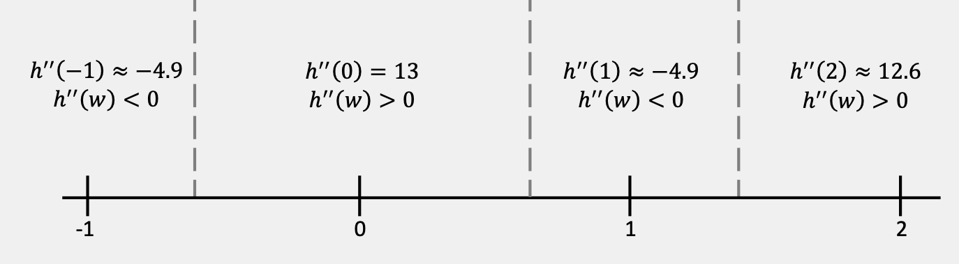
So we find that the intervals of concave up/concave down are
$$\require{bbox} \bbox[2pt,border:2px solid green]{\begin{array}{rc} \text{Concave up:} & (-0.6771, 0.6771), (1.4173,2]\\ \text{Concave down:} & [-1, -0.6771), (0.6771, 1.4173)\\ \end{array}}$$Be careful with the endpoints of these intervals. We are working on the interval $[-1,2]$ only. We have not considered any points outside of this interval, so we can't say anything about the concavity outside of the interval.
To answer this part, we need to interpret the results from part (b). Recall that an inflection point occurs where the concavity of the graph changes. Therefore, the inflection points for this function on this interval occur when
$$\require{bbox} \bbox[2pt,border:2px solid green]{w\approx -0.6771 \hspace{.2in} w\approx 0.6771 \hspace{.2in} w\approx 1.4173}$$As in part (b), we need to be careful and recall that we are working on the interval $[-1,2].$ There are infinitely many more possible inflection points, but since we have only worked within the interval $[-1,2],$ we cannot say whether or not they are inflection points.
We need the second derivative to find the possible inflection points, so here it is:
\begin{align*} R'(z) &= (z+4)^{\frac23} + z\left(\frac23\right) (z+4)^{-\frac13} = \frac{5z+12}{3(z+4)^{\frac13}}\\ R''(z) &= \frac{5\left(3(z+4)^{\frac13}\right)-(5z+12)(z+4)^{-\frac23}}{\left[ 3(z+4)^{\frac13}\right]^2}= \\ &=\frac{[15(z+4)-(5z+12)](z+4)^{-\frac23}}{9(z+4)^{\frac23}}= \frac{10z+48}{9(z+4)^{\frac43}}\\ \end{align*}Note that we simplified the derivatives at each stage. Having the second derivative in its simplest form will help us find the answer to this part.
Recall that the possible inflection points occur where the second derivative is either zero or does not exist. In the simplified form of the second derivative, we set the denominator and numerator equal to zero and solve for $z.$
We see that the second derivative does not exist at $z=-4,$ but that the original function does exist there. So $z=-4$ is the location of a possible inflection point. The second derivative is zero at $z=-\frac{48}{10}=-4.8,$ so that is another location of a possible inflection point.
$$\require{bbox} \bbox[2pt,border:2px solid green]{z=-\frac{48}{10}=-4.8 \hspace{.2in} \& \hspace{.2in} z=-4}$$We need the number line for the second derivative to answer this part. Here it is:
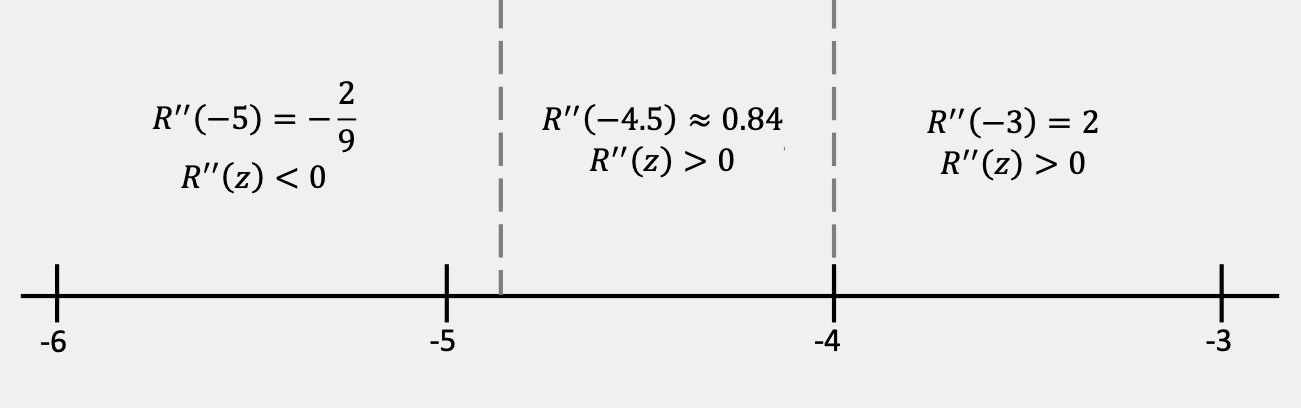
So we find that the intervals of concave up/concave down are
$$\require{bbox} \bbox[2pt,border:2px solid green]{\begin{array}{rc} \text{Concave up:} & (-4.8,-4), (-4,\infty)\\ \text{Concave down:} & (-\infty,-4.8)\\ \end{array}}$$To answer this part, we need to interpret the results from part (b). Recall that an inflection point occurs where the concavity of the graph changes. Therefore, the single inflection point for this function is located at $$\require{bbox} \bbox[2pt,border:2px solid green]{z=-4.8}$$
To find the locations of the possible inflection points, we need the second derivative. Here it is:
\begin{align*} h'(x) &= -2x\text{e}^{4-x^2}\\ h''(x) &= -2\text{e}^{4-x^2} + 4x^2\text{e}^{4-x^2} = 2\text{e}^{4-x^2}(2x^2-1)\\ \end{align*}The second derivative exists everywhere because exponential functions and polynomials exist everywhere. So we need to set the second derivative equal to zero and solve for $x$ to find the possible inflection points' locations. Notice that we have factored the exponential from both terms of the second derivative. This will make solving $h''(x)=0$ easier.
Recall that exponential functions are never zero, so the second derivative is zero when $$2x^2-1=0.$$
The locations of the possible inflection points are then
$$\require{bbox} \bbox[2pt,border:2px solid green]{x=\pm\frac{1}{\sqrt{2}}\approx \pm 0.7071}$$We need the number line for the second derivative to answer this part. Here it is:
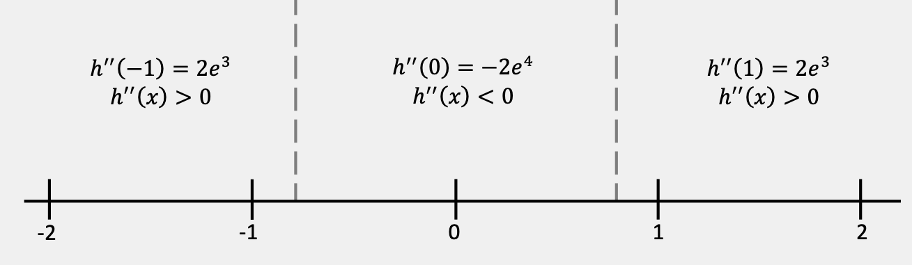
So we find that the intervals of concave up/concave down are
$$\require{bbox} \bbox[2pt,border:2px solid green]{\begin{array}{rc} \text{Concave up:} & \left(-\infty, -\frac{1}{\sqrt{2}}\right), \left(\frac{1}{\sqrt{2}},\infty\right)\\ \text{Concave down:} & \left(-\frac{1}{\sqrt{2}}, \frac{1}{\sqrt{2}}\right)\\ \end{array}}$$To answer this part, we need to interpret the results from part (b). Recall that an inflection point occurs where the concavity of the graph changes. Therefore, the inflection points for this function occur when
$$\require{bbox} \bbox[2pt,border:2px solid green]{x=-\frac{1}{\sqrt{2}}\approx -0.7071\hspace{.25in} x=\frac{1}{\sqrt{2}}\approx 0.7071}$$For the functions in problems 9 - 14, do the following:
- Identify the critical numbers of the function.
- Determine the intervals on which the function is increasing and those on which it is decreasing.
- Classify each critical point as a relative maximum, a relative minimum or neither.
- Determine the intervals on which the function is concave up and those on which it is concave down.
- Determine the inflection points of the function.
- Use the information from parts (a) - (e) to sketch the graph of the function.
- $g(t)=t^5-5t^4+8$
- $f(x)=5-8x^3-x^4$
- $h(z)=z^4-2z^3-12z^2$
- $Q(t)=3t-8\sin\left(\displaystyle\frac{t}{2}\right)$ on the interval $[-7,4]$
- $f(x)=x^{\frac43}(x-2)$
- $P(w)=w\text{e}^{4w}$
- Determine the minimum degree of a polynomial that has exactly one inflection point.
- Suppose that we know that $f(x)$ is a polynomial with critical numbers $x=-1, x=2$ and $x=6.$ Further suppose that the second derivative is $f''(x)=-3x^2+14x-4.$ If possible, classify each critical point as a relative minimum or a relative maximum. If it is not possible to classify the critical points, explain clearly why they cannot be classified.
Parts (a) - (e) of this problem are just like the increasing/decreasing problems from the previous section and the concavity problems from earlier in this section. Because of this, we won't be showing very much detail here. If you are unsure about how to approach any of the questions asked in parts (a) - (e), take a look at the problems in the previous section or earlier in this section before proceeding.
Solution to (a)
To find the critical numbers, we need the first derivative: $$g'(t) = 5t^4-20t^3=5t^3(t-4)$$ Setting the first derivative equal to zero, we find that the critical numbers are
$$\require{bbox} \bbox[2pt,border:2px solid green]{t=0\hspace{.2in}\&\hspace{.2in} t=4}$$Solution to (b)
Here is the number line for the first derivative:

From the number line, we find the following increasing/decreasing information for this function:
$$\require{bbox} \bbox[2pt,border:2px solid green]{\begin{array}{rl} \text{Increasing:} & (-\infty, 0)\hspace{.1in} \& \hspace{.1in}(4,\infty)\\ \text{Decreasing:} & (0,4)\\ \end{array}}$$Solution to (c)
Using the First Derivative Test and the number line above, we find the following classifications of the critical points.
$$\require{bbox} \bbox[2pt,border:2px solid green]{\begin{array}{rl} t=0: & \text{Relative Maximum}\\ t=4: & \text{Relative Minimum}\\ \end{array}}$$Solution to (d)
To find the list of possible inflection points, we need the second derivative. $$g''(t) = 20t^3-60t^2=20t^2(t-3)$$ Setting the second derivative equal to zero and solving for $x,$ we find that the possible inflection points occur at
$$\require{bbox} \bbox[2pt,border:2px solid green]{t=0\hspace{.1in}\&\hspace{.1in}t=3}$$To find the concavity information for this function, we need the number line for the second derivative. Here it is:

From the number line, we find the following concavity information for the function:
$$\require{bbox} \bbox[2pt,border:2px solid green]{ \text{Concave Up:}\hspace{.1in} (3,\infty)\hspace{.25in} \text{Concave Down:}\hspace{.1in} (-\infty, 0)\hspace{.1in} \& \hspace{.1in}(0,3)}$$Solution to (e)
Using the number line from the previous step, we see that the concavity changes once. The single inflection point occurs at
$$\require{bbox} \bbox[2pt,border:2px solid green]{t=3}$$Solution to (f)
As we did in problems in this section, we start at the left and work our way to the right on the graph. As we do this, we first pay attention to the increasing/decreasing information, and then we make sure that the curve has the correct concavity as we sketch it.

Note that because we used Geogebra to sketch this graph, it is possible that your sketch won't be exactly the same. It should, however, have the same points listed as on the graph above, the same basic increasing/decreasing nature, and the same basic concavity pattern.
Parts (a) - (e) of this problem are just like the increasing/decreasing problems from the previous section and the concavity problems from earlier in this section. Because of this, we won't be showing very much detail here. If you are unsure about how to approach any of the questions asked in parts (a) - (e), take a look at the problems in the previous section or earlier in this section before proceeding.
Solution to (a)
To find the critical numbers, we need the first derivative: $$f'(x) = -24x^2-4x^3=-4x^2(x+6)$$ Setting the first derivative equal to zero, we find that the critical numbers are
$$\require{bbox} \bbox[2pt,border:2px solid green]{x=-6\hspace{.2in}\&\hspace{.2in} x=0}$$Solution to (b)
Here is the number line for the first derivative:

From the number line, we find the following increasing/decreasing information for this function:
$$\require{bbox} \bbox[2pt,border:2px solid green]{\begin{array}{rl} \text{Increasing:} & (-\infty, -6)\\ \text{Decreasing:} & (-6,0)\hspace{.1in} \& \hspace{.1in} (0,\infty)\\ \end{array}}$$Solution to (c)
Using the First Derivative Test and the number line above, we find the following classifications of the critical points.
$$\require{bbox} \bbox[2pt,border:2px solid green]{\begin{array}{rl} x=-6: & \text{Relative Maximum}\\ x=0: & \text{Neither}\\ \end{array}}$$Solution to (d)
To find the list of possible inflection points, we need the second derivative. $$f''(x) = -48x-12x^2=-12x(x+4)$$ Setting the second derivative equal to zero and solving for $t,$ we find that the possible inflection points occur at
$$\require{bbox} \bbox[2pt,border:2px solid green]{x=-4\hspace{.1in} \&\hspace{.1in} x=0}$$To find the concavity information for this function, we need the number line for the second derivative. Here it is:
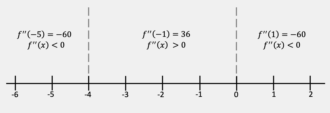
From the number line, we find the following concavity information for the function:
$$\require{bbox} \bbox[2pt,border:2px solid green]{ \text{Concave Up:}\hspace{.1in} (-4,0)\hspace{.25in} \text{Concave Down:}\hspace{.1in} (-\infty,-4)\hspace{.1in} \& \hspace{.1in}(0,\infty)}$$Solution to (e)
From the concavity information in the previous step, we find that the inflection points occur at
$$\require{bbox} \bbox[2pt,border:2px solid green]{x=-4\hspace{.1in}\&\hspace{.1in} x=0}$$Solution to (f)
As we did in problems in this section, we start at the left and work our way to the right on the graph. As we do this, we first pay attention to the increasing/decreasing information, and then we make sure that the curve has the correct concavity as we sketch it.

Note that because we used Geogebra to sketch this graph, it is possible that your sketch won't be exactly the same. It should, however, have the same points listed as on the graph above, the same basic increasing/decreasing nature, and the same basic concavity pattern.
Parts (a) - (e) of this problem are just like the increasing/decreasing problems from the previous section and the concavity problems from earlier in this section. Because of this, we won't be showing very much detail here. If you are unsure about how to approach any of the questions asked in parts (a) - (e), take a look at the problems in the previous section or earlier in this section before proceeding.
Solution to (a)
To find the critical numbers, we need the first derivative: $$h'(z) = 4z^3-6z^2-24z=2z(2z^2-3z-12)$$ Setting the first derivative equal to zero, we find that the critical numbers are
$$\require{bbox} \bbox[2pt,border:2px solid green]{z=0\hspace{.2in}\&\hspace{.2in} z=\frac{3\pm\sqrt{105}}{4}\approx-1.8117, 3.3117}$$Solution to (b)
Here is the number line for the first derivative:
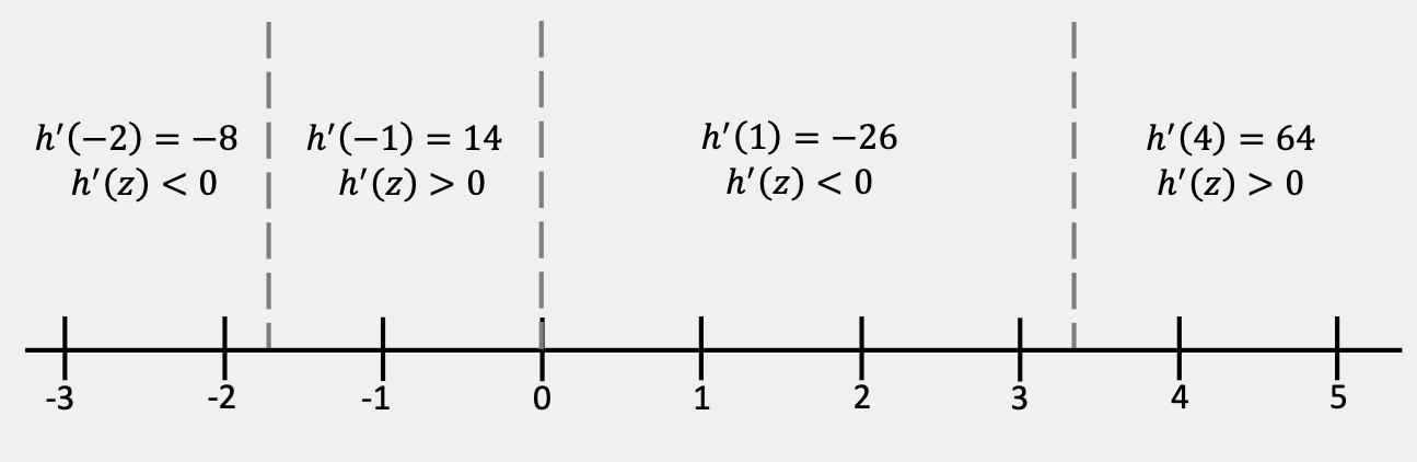
From the number line, we find the following increasing/decreasing information for this function:
$$\require{bbox} \bbox[2pt,border:2px solid green]{\begin{array}{rl} \text{Increasing:} & \left(\frac{3-\sqrt{105}}{4},0\right)\hspace{.1in}\&\hspace{.1in}\left(\frac{3+\sqrt{105}}{4},\infty\right)\\ \text{Decreasing:} & \left(-\infty, \frac{3-\sqrt{105}}{4}\right)\hspace{.1in} \& \hspace{.1in} \left(0,\frac{3+\sqrt{105}}{4}\right)\\ \end{array}}$$Solution to (c)
Using the First Derivative Test and the number line above, we find the following classifications of the critical points.
$$\require{bbox} \bbox[2pt,border:2px solid green]{\begin{array}{rl} z=\frac{3\pm\sqrt{105}}{4}: & \text{Relative Minimum}\\ z=0: & \text{Relative Maximum}\\ \end{array}}$$Solution to (d)
To find the list of possible inflection points, we need the second derivative. $$h''(z) = 12z^2-12z-24=12(z-2)(z+1)$$ Setting the second derivative equal to zero and solving for $z,$ we find that the possible inflection points occur at
$$\require{bbox} \bbox[2pt,border:2px solid green]{z=-1\hspace{.1in} \&\hspace{.1in} z=2}$$To find the concavity information for this function, we need the number line for the second derivative. Here it is:
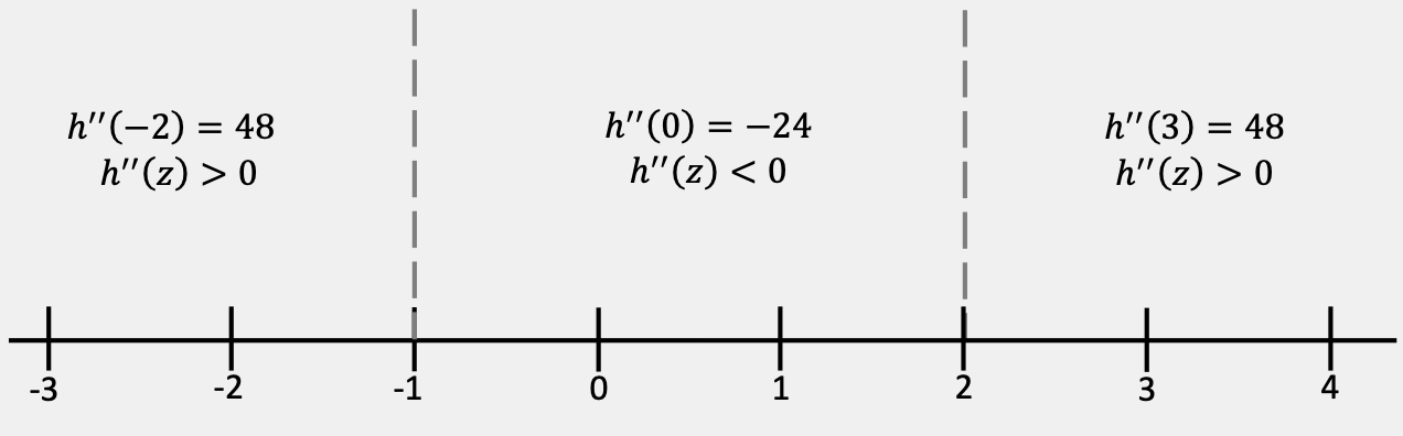
From the number line, we find the following concavity information for the function:
$$\require{bbox} \bbox[2pt,border:2px solid green]{ \text{Concave Up:}\hspace{.1in} (-\infty,-1)\hspace{.1in}\&\hspace{.1in}(2,\infty)\hspace{.25in} \text{Concave Down:}\hspace{.1in} (-1,2)}$$Solution to (e)
From the concavity information in the previous step, we find that the inflection points occur at
$$\require{bbox} \bbox[2pt,border:2px solid green]{z=-1\hspace{.1in}\&\hspace{.1in} z=2}$$Solution to (f)
As we did in problems in this section, we start at the left and work our way to the right on the graph. As we do this, we first pay attention to the increasing/decreasing information, and then we make sure that the curve has the correct concavity as we sketch it.

Note that because we used Geogebra to sketch this graph, it is possible that your sketch won't be exactly the same. It should, however, have the same points listed as on the graph above, the same basic increasing/decreasing nature, and the same basic concavity pattern.
Parts (a) - (e) of this problem are just like the increasing/decreasing problems from the previous section and the concavity problems from earlier in this section. Because of this, we won't be showing very much detail here. If you are unsure about how to approach any of the questions asked in parts (a) - (e), take a look at the problems in the previous section or earlier in this section before proceeding.
Solution to (a)
To find the critical numbers, we need the first derivative: $$Q'(t)=3-4\cos\left(\frac{t}{2}\right)$$
Then we need to solve the trigonometric equation
$$\cos\left(\frac{t}{2}\right) = \frac34$$The complete list of critical numbers is
$$\begin{array}{ll} t\approx 1.4454+4\pi n &\\ & n=0,\pm1,\pm2, \pm3, \ldots\\ t\approx 11.1210 + 4\pi n & \\ \end{array}$$After substituting values of $n,$ we find the critical numbers in the interval $[-7,4]$ are
$$\require{bbox} \bbox[2pt,border:2px solid green]{t\approx -1.4454\hspace{.1in} \& \hspace{.1in} t\approx 1.4454}$$Solution to (b)
Here is the number line for the first derivative:
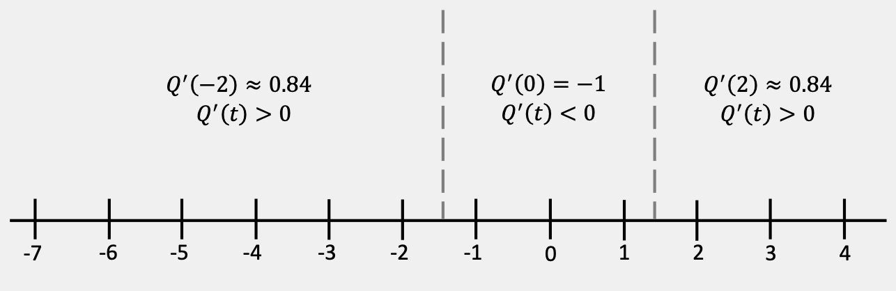
From the number line, we find the following increasing/decreasing information for this function:
$$\require{bbox} \bbox[2pt,border:2px solid green]{\begin{array}{rl} \text{Increasing:} & [-7,-1.44554)\hspace{.1in}\&\hspace{.1in} (1.4454,4]\\ \text{Decreasing:} & (-1.4454,1.4454)\\ \end{array}}$$Solution to (c)
Using the First Derivative Test and the number line above, we find the following classifications of the critical points.
$$\require{bbox} \bbox[2pt,border:2px solid green]{\begin{array}{rl} t\approx -1.4454: & \text{Relative Maximum}\\ t\approx 1.4454: & \text{Relative Minimum}\\ \end{array}}$$Solution to (d)
To find the list of possible inflection points, we need the second derivative.
$$Q''(t) = 2\sin\left(\frac{t}{2}\right)$$We need to set the second derivative equal to zero and solve for $t$ to find the list of possible inflection points. The complete list is
$$\begin{array}{ll} t=4\pi n & \\ & n=0, \pm1, \pm2, \pm3, \ldots\\ t=2\pi +4\pi n & \\ \end{array}$$After substituting some values of $n$ into the list above, we find that the possible inflection points in the interval $[-7,4]$ are located at
$$\require{bbox} \bbox[2pt,border:2px solid green]{t\approx -6.2832\hspace{.1in} \&\hspace{.1in} t=0}$$To find the concavity information for this function, we need the number line for the second derivative. Here it is:
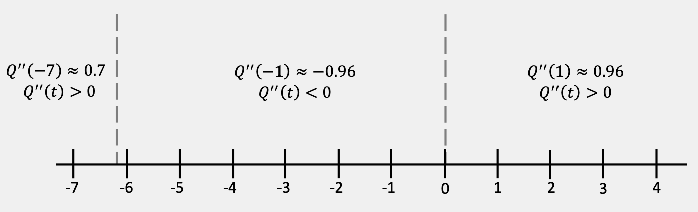
From the number line, we find the following concavity information for the function:
$$\require{bbox} \bbox[2pt,border:2px solid green]{ \text{Concave Up:}\hspace{.1in} [-7,-6.2832)\hspace{.1in}\&\hspace{.1in}(0,4]\hspace{.25in} \text{Concave Down:}\hspace{.1in} (-6.2832,0)}$$Solution to (e)
From the concavity information in the previous step, we find that the inflection points occur at
$$\require{bbox} \bbox[2pt,border:2px solid green]{t\approx -6.2832\hspace{.1in}\&\hspace{.1in} t=0}$$Solution to (f)
As we did in problems in this section, we start at the left and work our way to the right on the graph. As we do this, we first pay attention to the increasing/decreasing information, and then we make sure that the curve has the correct concavity as we sketch it.

Note that because we used Geogebra to sketch this graph, it is possible that your sketch won't be exactly the same. It should, however, have the same points listed as on the graph above, the same basic increasing/decreasing nature, and the same basic concavity pattern.
Parts (a) - (e) of this problem are just like the increasing/decreasing problems from the previous section and the concavity problems from earlier in this section. Because of this, we won't be showing very much detail here. If you are unsure about how to approach any of the questions asked in parts (a) - (e), take a look at the problems in the previous section or earlier in this section before proceeding.
Solution to (a)
To find the critical numbers, we need the first derivative: $$f'(x) = \frac73 x^{\frac43}-\frac83 x^{\frac13} = \frac13 x^{\frac13}(7x-8)$$ Setting the first derivative equal to zero, we find that the critical numbers are
$$\require{bbox} \bbox[2pt,border:2px solid green]{x=0\hspace{.2in}\&\hspace{.2in} x=\frac87\approx 1.1429}$$Solution to (b)
Here is the number line for the first derivative:

From the number line, we find the following increasing/decreasing information for this function:
$$\require{bbox} \bbox[2pt,border:2px solid green]{ \text{Increasing:}\hspace{.1in} (-\infty,0)\hspace{.1in}\&\hspace{.1in} \left(\frac87,\infty\right)\hspace{.25in} \text{Decreasing:}\hspace{.1in} \left(0, \frac87\right)}$$Solution to (c)
Using the First Derivative Test and the number line above, we find the following classifications of the critical points.
$$\require{bbox} \bbox[2pt,border:2px solid green]{\begin{array}{rl} x=0: & \text{Relative Maximum}\\ x=\frac87: & \text{Relative Minimum}\\ \end{array}}$$Solution to (d)
To find the list of possible inflection points, we need the second derivative.
$$f''(x) = \frac{28}{9}x^{\frac13}-\frac89 x^{-\frac23} = \frac{28x-8}{9x^{\frac23}}$$The possible inflection points occur where the second derivative is zero or undefined. Setting both numerator and denominator equal to zero and solving for $x,$ we find that the possible inflection points for this function are located at
$$\require{bbox} \bbox[2pt,border:2px solid green]{x=0\hspace{.1in} \&\hspace{.1in} x=\frac27\approx 0.2857}$$To find the concavity information for this function, we need the number line for the second derivative. Here it is:

Using the number line, we find the following concavity information for the function:
$$\require{bbox} \bbox[2pt,border:2px solid green]{ \text{Concave Up:}\hspace{.1in} \left(\frac27,\infty\right)\hspace{.25in} \text{Concave Down:}\hspace{.1in} (-\infty,0)\hspace{.1in}\&\hspace{.1in} \left(0,\frac27\right)}$$Solution to (e)
From the concavity information in the previous step, we find that the only inflection point occurs at
$$\require{bbox} \bbox[2pt,border:2px solid green]{x=\frac27}$$Solution to (f)
As we did in problems in this section, we start at the left and work our way to the right on the graph. As we do this, we first pay attention to the increasing/decreasing information, and then we make sure that the curve has the correct concavity as we sketch it.

Note that because we used Geogebra to sketch this graph, it is possible that your sketch won't be exactly the same. It should, however, have the same points listed as on the graph above, the same basic increasing/decreasing nature, and the same basic concavity pattern.
Parts (a) - (e) of this problem are just like the increasing/decreasing problems from the previous section and the concavity problems from earlier in this section. Because of this, we won't be showing very much detail here. If you are unsure about how to approach any of the questions asked in parts (a) - (e), take a look at the problems in the previous section or earlier in this section before proceeding.
Solution to (a)
To find the critical numbers, we need the first derivative:
$$P'(w) = \text{e}^{4w}+4w\text{e}^{4w} = \text{e}^{4w}(1+4w)$$Since the exponential function is defined everywhere, the only critical number occurs where the first derivative is zero:
$$\require{bbox} \bbox[2pt,border:2px solid green]{w=-\frac14}$$Solution to (b)
Here is the number line for the first derivative:

From the number line, we find the following increasing/decreasing information for this function:
$$\require{bbox} \bbox[2pt,border:2px solid green]{ \text{Increasing:}\hspace{.1in}\left(-\frac14,\infty\right)\hspace{.25in} \text{Decreasing:} \hspace{.1in} \left(-\infty, -\frac14\right)}$$Solution to (c)
Using the First Derivative Test and the number line above, we find the following classification of the critical point.
$$\require{bbox} \bbox[2pt,border:2px solid green]{ w=-\frac14:\hspace{.1in} \text{Relative Minimum}}$$Solution to (d)
To find the list of possible inflection points, we need the second derivative.
$$P''(w) = \text{e}^{4w}(4)+4\text{e}^{4w}(1+4w) = 8\text{e}^{4w}(1+2w)$$Since the exponential function is defined everywhere, the only possible critical point is at
$$\require{bbox} \bbox[2pt,border:2px solid green]{w=-\frac12}$$To find the concavity information for this function, we need the number line for the second derivative. Here it is:

From the number line, we find the following concavity information for the function:
$$\require{bbox} \bbox[2pt,border:2px solid green]{ \text{Concave Up:}\hspace{.1in} \left(-\frac12,\infty\right)\hspace{.25in} \text{Concave Down:}\hspace{.1in} \left(-\infty,-\frac12\right)}$$Solution to (e)
From the concavity information in the previous step, we find that the only inflection point occurs at
$$\require{bbox} \bbox[2pt,border:2px solid green]{w=-\frac12}$$Solution to (f)
As we did in problems in this section, we start at the left and work our way to the right on the graph. As we do this, we first pay attention to the increasing/decreasing information, and then we make sure that the curve has the correct concavity as we sketch it.

Note that because we used Geogebra to sketch this graph, it is possible that your sketch won't be exactly the same. It should, however, have the same points listed as on the graph above, the same basic increasing/decreasing nature, and the same basic concavity pattern.
We should also note here that the behavior of the graph as $w\to \pm\infty$ might be a little tricky to figure out. To actually take those limits, we need a limit rule, L'Hôpital's Rule, that we will cover in a future section. Once we have covered that section, you should come back to this graph and see if you agree with the end behavior of the graph that is shown.
First, let's suppose that the single inflection point occurs at $x=a$ for some number $a.$ The value of $a$ is not important, this just allows us to discuss the question.
The function we're talking about is a polynomial, so let's call it $p(x).$ Since every derivative of a polynomial is also a polynomial, we know that the first and second derivatives, $p'(x)$ and $p''(x),$ are polynomials. Since there is an inflection point at $x=a,$ we know that $p''(a)=0$ and that the second derivative changes sign at $x=a.$
The simplest polynomial that equals zero at $x=a$ is $p''(x)=x-a.$ We notice that this function also changes sign at $x=a,$ so it fits our two requirements for the second derivative. Note that we don't really care on which side the graph is concave up and concave down, we just need the concavity to change at $x=a.$
Now that we have the second derivative, we can work back to the original function. We don't need the actual function, though, we just need its degree. So we don't have to completely "undo" the derivatives, we just need to think about how the degree changes as we take derivatives.
When we use the power rule to take the derivative of a polynomial, the degree decreases by one. Here we have a second derivative that is degree 1, and that degree is one lower than the degree of the first derivative. That means that $p'(x)$ must be a polynomial of degree 2. Using similar reasoning, we find that the original function must be a polynomial of degree 3.
So the minimum degree of a polynomial that has exactly one inflection point is three, a cubic polynomial.
Note that there are higher degree polynomials with exactly one inflection point, too. But there are no second or first degree polynomials with this property.
This problem might sound difficult at first, but since we've been given the second derivative, we might be able to use the Second Derivative Test to classify the critical numbers.
We should first note that because we were told that $f(x)$ is a polynomial, its first derivative is also a polynomial and is therefore defined everywhere. That means that whatever $f'(x)$ is, we have
$$f'(-1)=0\hspace{.2in} f'(2)=0\hspace{.2in} f'(6)=0$$This means that we can use the Second Derivative Test on these critical numbers. (Recall that the test only works on this type of critical number.)
Now to use the Second Derivative Test, we need to evaluate the second derivative at each of the critical numbers. Then, as long as the result isn't zero, the sign of the result tells us what type of critical point is at each of the critical numbers.
$$\require{bbox} \bbox[2pt,border:2px solid green]{\begin{array}{ll} f''(-1)=-21<0 & \text{Relative Maximum}\\ f''(2) = 12>0 & \text{Relative Minimum}\\ f''(6) = -28<0 & \text{Relative Maximum}\\ \end{array}}$$Assignment Problems
For problems 1 & 2 the graph of a function is given. Determine the intervals on which the function is concave up and those on which it is concave down.


For problems 3 - 5, the graph of the second derivative of a function is given. From the graph, determine the intervals on which the original function is concave up and the intervals on which it is concave down.


For the functions in problems 6 - 18, determine the following:
- The intervals on which the function is concave up and those on which it is concave down.
- The inflection points of the function.
- $f(x)=x^3+9x^2+24x-6$
- $Q(t)=t^4-2t^3-120t^2-84t+35$
- $h(z)=3z^5-20z^4+40z^3$
- $g(w)=5w^4-2w^3-18w^2+108w-12$
- $g(x)=10+360x+20x^4+3x^5-x^6$
- $A(x)=9x-3x^2-160\sin\left(\displaystyle\frac{x}{4}\right)$ on the interval $[-20,11]$
- $f(x)=3\cos(2x)-x^2-14$ on the interval $[0,6]$
- $h(t)=1+2t^2-\sin(2t)$ on the interval $[-2,4]$
- $R(v)=v(v-8)^{\frac13}$
- $g(x)=(x-1)(x+3)^{\frac25}$
- $f(x)=\text{e}^{4x}-\text{e}^{-x}$
- $h(w)=w^2\text{e}^{-w}$
- $A(w)=w^2-\ln(w^2+1)$
For the functions in problems 19 - 33, do the following:
- Identify the critical numbers of the function.
- Determine the intervals on which the function is increasing and those on which it is decreasing.
- Classify each critical point as a relative minimum, a relative maximum or neither.
- Determine the intervals on which the function is concave up and those on which it is concave down.
- Determine the inflection points of the function.
- Use the information from parts (a) - (e) to sketch the graph of the function.
- $f(x)=10-30x^2+2x^3$
- $G(t)=14+4t^3-t^4$
- $h(w)=w^4+4w^3-18w^2-9$
- $g(z)=10z^3+10z^4+3z^5$
- $f(z)=z^6-9z^5+20z^4+10$
- $Q(t)=3t-5\sin(2t)$ on the interval $[-1,4]$
- $g(x) = \displaystyle\frac12 x+\cos\left(\displaystyle\frac{x}{3}\right)$ on the interval $[-25,0]$
- $h(x) = x(x-4)^{\frac13}$
- $f(t)=t\sqrt{t^2+1}$
- $A(z)=z^{\frac45}(z-27)$
- $g(w)=\text{e}^{4w}-\text{e}^{6w}$
- $P(t) = 3t\text{e}^{1-\frac14 t^2}$
- $g(x) = (x+1)^3\text{e}^{-x}$
- $h(z)=\ln(z^2+z+1)$
- $f(w)=2w-8\ln(w^2+4)$
- Answer each of the following questions:
- What is the minimum degree of a polynomial that has exactly two inflection points?
- What is the minimum degree of a polynomial that has exactly three inflection points?
- What is the minimum degree of a polynomial that has exactly $n$ inflection points?
- Suppose that for some function $f(x),$ it is known that there is an inflection point at $x=3.$ Answer each of the following questions about this function.
- What is the simplest form that the second derivative of this function can have?
- Using your answer to part (a), determine the most general form that the function itself can have.
- Given that $f(0) = - 6$ and $f(3)=1,$ find a specific function that has an inflection point at $x=3.$
In problems 36 - 39, assume that $f(x)$ is a polynomial. Use the given second derivative of the function to classify, if possible, each of the given critical numbers as corresponding to a relative minimum or a relative maximum. If it is not possible to classify a critical point, explain clearly why it cannot be classified.
- $f''(x)=3x^2-4x-15.$ The critical numbers are $x=-3, x=0$ and $x=5.$
- $f''(x)=4x^3-21x^2-24x+68.$ The critical numbers are $x=-2, x=4$ and $x=7.$
- $f''(x)=23+18x-9x^2-4x^3.$ The critical numbers are $x=-4, x=-1$ and $x=3.$
- $f''(x)=216-410x+249x^2-60x^3+5x^4.$ The critical numbers are $x=1, x=4$ and $x=5.$
- Use the function $f(x)=(x+1)^3(x-1)^4$ for this problem.
- Determine the critical numbers of the function.
- Use the Second Derivative Test to classify each critical point as a relative minimum or a relative maximum. If it is not possible to classify a critical point, explain clearly why it cannot be classified.
- Use the First Derivative Test to classify each critical point as a relative minimum, a relative maximum or neither.
- Suppose that the graphs of $f(x)$ and $g(x)$ are concave down. Define $h(x) = f(x) + g(x)$ and show that the graph of $h(x)$ is also concave down.
- Suppose that the graph of $f(x)$ is concave up. Let $h(x) = f(x) + g(x)$ for some function $g(x).$ Determine a condition on $g(x)$ under which the graph of $h(x)$ will be concave up.
- Let $f(x)$ be a function and define $h(x) = [f(x)]^2.$ Determine conditions on $f(x)$ under which the graph of $h(x)$ will be concave up. Note that there are several sets of conditions that will work here. How many can you find?
Note: The following content is adapted from OpenStax and is licensed under a Creative Commons Attribution-NonCommercial-ShareAlike 4.0 International License.
Access for free at https://openstax.org/books/calculus-volume-1/pages/1-introduction.
In problems 44 - 48, there is a sentence describing some function. Interpret the sentence in terms of $f$, $f',$ and $f''.$
- The population is growing more slowly. Here, $f$ is the population.
- A bike accelerates faster, but a car goes faster. Here, $f =$ bike's position minus car's position.
- The airplane lands smoothly. Here, $f$ is the plane's altitude.
- Stock prices are at their peak. Here, $f$ is the stock price.
- The economy is picking up speed. Here, $f$ is a measure of the economy, such as GDP.
For problems 49 - 53, consider a third-degree polynomial $f(x),$ which has the properties $$f'(1)=0, f'(3)=0$$ Determine whether the following statements are true or false. Justify your answer.
- $f(x)=0$ for some $1\leq x\leq 3.$
- $f''(x)=0$ for some $1\leq x\leq 3.$
- There is no absolute maximum at $x=3.$
- If $f(x)$ has three real zeros, then it has one inflection point.
- If $f(x)$ has one inflection point, then it has three real zeros.